How to stabilize daily transport reliability: a 4-lens playbook turning CET/CPK into predictable attendance
This is an operational playbook, not a sales pitch. It translates CET/CPK metrics, seat-fill, and dead-mile reduction into concrete guardrails and SOP-level steps that dispatch and vendor teams can execute during peak and crisis conditions. You'll find crisp escalation paths, data trails, and proven controls designed to reduce firefighting and give the control-room a quiet, steady rhythm.
Is your operation showing these patterns?
- Escalations spike at night during festival weeks or monsoon disruptions
- Route changes occur without documented approvals, triggering extra dead miles
- Seat-fill appears to improve on paper while attendance remains volatile
- Vendor responses lag beyond SLA during outages
- GPS logs show gaps or inconsistent traces during peak shifts
- Toil in month-end reconciliation grows month over month
Operational Framework & FAQ
stability & predictability in peak shifts
Build a control-room playbook to anticipate disruptions, triage alerts, and recover gracefully without escalating into crisis mode.
In our employee transport program, what does “cost & productivity linkage” really mean, and how do CET/CPK, seat-fill, and dead miles connect to attendance and shift adherence?
B0285 Define cost-to-productivity linkage — In India corporate Employee Mobility Services (EMS), what does “cost & productivity linkage” actually mean in practice, and how do CET/CPK, seat-fill ratio, and dead-mile reduction translate into measurable attendance stability and shift adherence?
Cost and productivity linkage in Indian Employee Mobility Services means that commute unit-economics (CET, CPK, seat-fill, dead miles) are managed specifically to protect on-time performance, attendance stability, and shift adherence, rather than as isolated transport KPIs. In mature EMS programs, every rupee saved or spent in the route model is tied back to whether employees arrive on time, every day, with minimal volatility.
Cost per Employee Trip (CET) and Cost per Kilometer (CPK) become useful only when they sit alongside On-Time Performance and Trip Adherence Rate. Low CET with poor OTP usually indicates under-capacity, weak buffers, or over-aggressive routing. That pattern often leads to late logins, manager escalations, and higher hidden productivity cost than the nominal saving on CET.
Seat-fill ratio and dead-mile reduction drive both unit cost and reliability. Higher seat-fill on pooled routes spreads fixed costs but needs careful shift windowing, so the algorithm does not create excessively long detours that erode punctuality. Dead-mile reduction lowers CPK and releases fleet capacity, which can then be redeployed as standby buffers or peak-hour extras to stabilize on-time pickups.
In practice, cost–productivity linkage is operationalized by tracking a small set of paired metrics per shift window, such as:
- CET and CPK mapped against OTP% and Trip Adherence Rate.
- Seat-fill ratio mapped against average ride time and late-login incidents.
- Dead mileage mapped against spare capacity and exception-closure time.
Most organizations that treat commute as an input to workforce productivity track attendance volatility and no-show rate by transport route. They then tune routing, fleet mix, and shift-aligned capacity so that cost curves and productivity curves improve together, rather than trading one off blindly against the other.
Why should Finance look at CET/CPK and dead miles as a productivity issue, not just a cab cost?
B0286 Why finance links cost to productivity — In India corporate ground transportation for shift-based employee commute (EMS), why do finance teams treat CET/CPK and dead miles as a productivity problem rather than just a transport cost line item?
Finance teams in India treat cost per employee trip (CET), cost per kilometre (CPK), and dead mileage as productivity problems because these metrics directly influence attendance, shift adherence, and overall output, not just the transport budget. Poorly managed CET/CPK and high dead miles usually signal unreliable routes, under-filled vehicles, and fragmented vendors, which translate into late logins, lost production hours, and extra supervisory effort every day.
Finance leaders see that high CET with unstable CPK often correlates with low vehicle utilization and inconsistent on-time performance. This pattern forces HR and operations into constant firefighting, which erodes productivity and creates more indirect cost than the transport line item itself. Dead mileage is treated as a pure waste multiplier, because it consumes budget without moving any employee and usually comes from inefficient routing, poor shift windowing, or weak vendor governance.
In EMS, mobility is tightly coupled with workforce productivity, so Finance tends to read transport data together with HRMS attendance, shift-roster patterns, and SLA reports. When CET/CPK improve through better seat-fill, routing, and central command-center control, Finance sees fewer exceptions, smoother audits, and more predictable unit economics. When they worsen, Finance expects to see impacts in overtime, attrition, and missed targets, so they frame these metrics as levers for operational efficiency rather than just as transport expenses.
At a high level, how should we measure seat-fill and dead miles consistently across vendors/sites so Ops and Finance stop debating definitions every month?
B0287 How to measure seat-fill and dead miles — In India enterprise employee transport operations (EMS), at a high level, how do you measure seat-fill ratio and dead-mileage consistently across vendors and sites so that Operations and Finance aren’t arguing about definitions every month?
For India enterprise employee transport operations, seat-fill ratio and dead mileage are measured consistently only when organizations define standard trip-level metrics, capture them from a single mobility data model, and lock these definitions into contracts, SOPs, and dashboards used by all vendors and sites. Operations and Finance alignment improves when every kilometer and every seat is tagged to a common trip ledger and reconciled against the same rules for “billable,” “utilized,” and “empty” movement.
Seat-fill ratio measurement starts at the trip manifest. Each trip is defined with a fixed seat capacity and a passenger manifest that is synchronized with HRMS rosters. The seat-fill ratio is then calculated per trip as occupied seats divided by total available seats. The same logic is rolled up per route, shift window, vendor, and site by using the underlying trip-level records rather than vendor summaries.
Dead mileage measurement depends on clean separation of loaded versus empty kilometers in telematics data. Each vehicle’s movement is split into segments such as garage-to-first-pickup, between last-drop-to-garage, inter-trip repositioning, and loaded route segments. Only segments with at least one manifested passenger on board are treated as productive kilometers. All other segments are tagged as dead mileage and then aggregated per vendor, route, and site for comparison.
To avoid monthly disputes, organizations codify these definitions in EMS contracts, vendor governance frameworks, and mobility dashboards. The same trip ledger and KPI library are exposed to Operations and Finance, so cost per kilometer, cost per employee trip, and trip fill ratio are computed once and reused everywhere. This shared semantic layer also supports outcome-linked procurement, unified command center monitoring, and emission calculations for ESG reporting.
images:
What are the common leakage points that mess up CET/CPK (dead miles, duplicates, no-shows, exceptions), and what controls catch them without slowing Ops down?
B0288 Leakage sources and practical controls — In India corporate Employee Mobility Services (EMS), what are the most common “leakage sources” that break the CET/CPK math (for example dead-mile inflation, duplicate trips, no-shows, route exceptions), and what controls typically catch them without creating operational drag?
The most common leakage sources in India EMS are dead mileage, low seat-fill, ungoverned exceptions, and weak trip-level verification, and the least painful controls are those embedded in routing engines, apps, and command-center workflows instead of manual checks. Leakage falls when CET/CPK math is tied to OTP, trip adherence, and audit-ready data rather than just vendor-reported kilometers.
Dead-mile inflation usually comes from poor shift windowing, ad-hoc cab releases, and vehicles running empty to or from low-utilization zones. Dynamic routing with dead-mile caps, fleet tagging by hub, and command-center route adherence audits reduce this, especially when vendor payments are indexed to optimized route kilometers instead of raw odometer readings.
Duplicate or “ghost” trips often appear when rosters change late or when app attendance is not enforced. Trip-level OTP or QR-based boarding, passenger manifest sync with HRMS, and a Trip Adherence Rate (TAR) KPI catch these silently. A common pattern is to only pay for trips with valid employee check-in plus GPS trace and a closed duty slip.
No-shows, partial loads, and chronic low seat-fill increase CET even when CPK looks fine. Seat-fill targets, pooled routing by shift band, and Trip Fill Ratio (TFR) reviews in monthly dashboards highlight this leakage. Outcome-based commercials where the vendor shares upside on utilization, but is capped on under-filled routes, prevent over-fleeting.
Route exceptions and manual overrides are a frequent blind spot. Geo-fencing, exception tagging in the driver app, and an approval workflow for off-route detours let Transport Heads allow genuine deviations without losing control of the audit trail. This keeps Security and EHS satisfied without adding call-based approvals that slow the operation.
Billing mismatches arise when trip data, GPS logs, and invoices are not reconciled to the same source of truth. A centralized mobility data lake or single NOC dashboard that feeds both MIS and billing, combined with automated tariff mapping and SLA-linked invoice checks, removes most manual reconciliation while keeping Finance in control.
How can our Transport/Facilities team quickly tell if low seat-fill is due to roster changes, bad routing, policy constraints, or vendor execution—and what minimum data is enough?
B0289 Diagnose drivers of low seat-fill — In India shift-based employee transport (EMS), how can a Transport/Facilities Head diagnose whether low seat-fill is caused by roster volatility, route design, policy constraints (women-first/night rules), or vendor execution—and which data points are enough to decide without a long consulting exercise?
In Indian shift-based employee transport, a Transport or Facilities Head can usually diagnose low seat-fill by checking a small, focused set of operational and policy data rather than running a long consulting exercise. The most reliable approach is to compare how seats, rosters, and policy rules behave over a few weeks of trips and see where the patterns break against expected benchmarks.
To distinguish roster volatility from other causes, operations teams should track planned versus actual headcount per shift, per route, and per day. A high gap between rostered employees and actual boarded employees, combined with frequent last-minute roster changes, indicates roster volatility is the primary driver. Roster volatility will usually show as many under-filled cabs across different vendors and routes, independent of location or timeband.
To test whether route design is the problem, teams should examine per-route seat-fill percentages, dead mileage, and trip adherence. Persistently low utilization on specific corridors or timebands, despite stable rosters, signals inefficient route design. This is especially clear when the same locations keep getting partly filled vehicles and when pooling logic does not align well with cluster density or shift windowing.
Policy constraints such as women-first rules and night-shift safety protocols can be identified by comparing seat-fill and routing behavior between policy-constrained trips and unconstrained trips. If cabs serving night shifts or women-first routes show systematically lower seat-fill and higher dead mileage than equivalent day or mixed-gender routes, policy constraints are a primary driver. This pattern will often correlate with mandatory escort requirements, geo-fencing restrictions, and female-first routing rules.
Vendor execution issues are usually visible when the roster, routes, and policies are stable but actual operations deviate. Signs include frequent last-minute vehicle substitutions, no-shows, unexplained trip cancellations, and poor on-time performance. Low seat-fill tied to vendor execution will often correlate with drivers refusing pooled pickups, partial route completion, or vehicles being dispatched late from the garage even when the manifest is full.
A Transport or Facilities Head does not need exhaustive analysis to reach a working diagnosis. A short, time-bound pull of the following data points over two to four weeks is usually enough:
- Planned versus boarded employees per shift, per route.
- Per-route seat-fill percentage and dead mileage.
- Breakdown of trips by policy category such as women-only, night shift, and escort-mandated.
- On-time performance and trip adherence rate across vendors, routes, and timebands.
- Vendor-wise exception logs including no-shows, route cut-short events, and repeated escalation patterns.
Combining these few metrics inside a command center-style dashboard allows the Transport or Facilities Head to see whether the core problem sits in roster behavior, routing design, safety policy structure, or vendor reliability. This focused diagnostic approach supports faster decisions on whether to change routing logic, renegotiate policies, re-educate employees, or escalate with vendors, and it keeps the daily control-room environment more predictable and less reactive.
What’s a realistic, audit-friendly way to connect dead-mile reduction to EBITDA when hybrid attendance keeps changing?
B0290 Audit-friendly EBITDA linkage under hybrid — In India corporate ground transport for employees (EMS), what is a realistic, auditable way for a CFO to link dead-mile reduction initiatives to EBITDA impact when attendance patterns change due to hybrid work?
A CFO can link dead-mile reduction to EBITDA by first defining a clean per-km cost baseline, then separately tracking “paid but unproductive” kilometres and tying every km saved—via routing and policy changes—to a reconciled reduction in total transport spend. The link holds only if dead-mile cuts are measured against stable unit economics, clean trip logs, and are adjusted for hybrid-work-driven volume changes.
A realistic approach starts with trip-level observability. Organizations need GPS or telematics-backed trip ledgers with clear tags for revenue/servicing km, dead mileage, and cancelled/no-show trips. These should be reconciled monthly with vendor invoices and internal HRMS or roster data to avoid misattributing reductions that are actually due to fewer shifts or lower headcount. CFOs should insist that Employee Mobility Services vendors provide dead-mile KPIs like dead-mile km per trip, dead-mile share of total km, and cost per employee trip (CET), with before/after comparisons aligned to the same attendance pattern or normalized per shift.
Hybrid work complicates attribution because attendance varies by day, shift window, and site. The CFO’s control is to normalize transport economics around unit views such as CET at a given average seat-fill and Vehicle Utilization Index. Dead-mile reduction should then be expressed as: “At the same average attendance and route pattern, route optimization and fleet mix changes reduced dead-mile share from X% to Y%, lowering CET by ₹Z.” Only this normalized delta should feed into the EBITDA bridge.
To make the impact auditable, Finance can embed dead-mile metrics into governance. This includes codifying them in SLAs, outcome-based commercials, and QBR dashboards. Dead-mile and CET should tie directly into cost-per-km (CPK), Utilization Revenue Index, and SLA breach penalties or incentives. Internal audit should be able to sample trip logs, GPS evidence, and invoices to confirm that dead-mile reductions correspond to lower billed km or lower effective CET, rather than being offset by added fixed fees or hidden minimum guarantees.
The EBITDA linkage then becomes a standard line in the P&L bridge: “Route and fleet optimization reduced dead-mile share by X percentage points at constant attendance, delivering ₹A million annualized reduction in EMS spend, net of any technology or vendor costs.” This can be cross-checked against broader mobility KPIs such as Trip Fill Ratio, OTP%, and complaint volumes to ensure that cost gains did not degrade reliability or employee experience, which would later show up as productivity or attrition costs.
How should HR and Finance agree on whether better OTP is actually improving attendance, or if we’re just adding buffers and raising CPK?
B0291 Separate real OTP gains from cost padding — In India Employee Mobility Services (EMS), how should HR and Finance agree on whether improved on-time pickup (OTP) is driving attendance stability versus just masking issues with longer buffers and higher CPK?
In India Employee Mobility Services, HR and Finance should jointly treat on-time pickup (OTP), attendance, and cost per km (CPK) as linked metrics, and then test whether OTP gains come from true routing efficiency or from hidden buffers and excess fleet. HR and Finance can align by defining a few shared KPIs, running time-bound experiments, and insisting on data that separates genuine reliability improvement from costlier over-padding of reporting times and routes.
HR teams typically see OTP through the lens of attendance stability, manager complaints, and employee sentiment. Finance teams look at OTP through CPK, cost per employee trip, dead mileage, and fleet utilization. A common failure mode is “buying OTP” through bigger time buffers, extra standby vehicles, and looser shift windows. This often improves OTP% but pushes CPK and CET up, with no real gain in productivity or commute experience.
The joint solution is to agree on a small, shared scoreboard that is reviewed together. At minimum, this scoreboard should track OTP%, no‑show rate, trip adherence rate, cost per employee trip, and trip fill ratio for the same time period and set of routes. HR should bring data from HRMS on late logins, shrinkage, and transport-linked grievances. Finance should bring aggregated billing and cost breakdowns mapped to those same shifts and sites.
Once this shared view exists, HR and Finance can run structured A/B style changes. For example, they can tighten buffers on a subset of routes while keeping fleet size constant. They should watch if OTP falls sharply and if attendance or complaints worsen. If OTP holds while buffers reduce and CPK stays flat or improves, that indicates true routing efficiency rather than masking. If OTP is “high” only when buffers and spare vehicles are high, the cost of that strategy becomes visible and negotiable.
To avoid blaming each other, both teams should insist that any EMS vendor or platform provide transparent routing and cost analytics rather than just headline OTP. HR should ask how route optimization, real-time tracking, and hybrid-work rostering are reducing dead mileage and idle time. Finance should ask to see OTP and CPK together, with clear evidence of seat-fill and dead mileage trends before and after changes. This approach aligns with outcome-linked procurement, where payouts are indexed not only to OTP but also to seat-fill and utilization, making it harder to win by over-padding.
A practical review cadence helps. A monthly HR–Finance–Transport review that looks at three clusters together is effective: reliability (OTP, TAR, exception closure time), experience (complaints, CEI-type scores, attrition signals), and economics (CPK, CET, utilization). If OTP improves without a corresponding reduction in late logins, absenteeism, or complaints, HR can call out “cosmetic OTP.” If OTP improves while CET and dead mileage spike, Finance can flag that buffers are too generous.
In mature EMS setups, the transport or facility head and the centralized command center are important allies. They can show whether OTP gains are coming from better dynamic routing and early alerts, or from over‑conservative planning. HR and Finance should lean on these operational insights before deciding which levers to institutionalize in contracts and SLAs.
What sensitivity checks should we run for festivals and monsoons so CET/CPK doesn’t blow up and we don’t get 3 a.m. route failure escalations?
B0292 Festival and monsoon sensitivity checks — In India shift-commute EMS operations, what sensitivity analyses do buyers typically run for festival seasons and monsoon disruptions to avoid budget surprises in CET/CPK and to prevent 3 a.m. escalation spikes from route failures?
In India shift-commute EMS operations, buyers typically run sensitivity analyses around demand spikes, capacity loss, and reliability degradation during festival seasons and monsoon to protect cost per employee trip (CET) and cost per kilometer (CPK), and to keep 3 a.m. escalations within defined thresholds. They stress-test routing, fleet mix, and vendor/NOC responsiveness against worst-case attendance, traffic, and weather patterns because reliability, safety, and cost predictability are tightly coupled in these periods.
During festival seasons, organizations model attendance volatility and shift-window compression. They test CET impact if seat-fill drops due to partial shifts, optional WFH, or late roster changes. Transport heads evaluate how many “thin” routes emerge and what happens to CPK when cabs run under-occupied. Procurement and Finance simulate alternate commercial constructs like per-seat vs per-trip, dead-mile caps, and peak-day surcharges to understand exposure. They also check whether centralized booking and approval workflows in EMS platforms can enforce cut-off times and roster-freeze rules, which reduces last-minute manual routing and escalation risk.
For monsoon disruptions, buyers run scenario tests on route adherence and on-time performance (OTP) under heavy traffic and waterlogging. They use historical traffic and incident data where available, or vendor case studies that demonstrate dynamic routing under adverse weather, such as the Mumbai monsoon example achieving a 98% on-time arrival rate and a 10% increase in customer satisfaction. Transport and Security teams stress-test business continuity plans and 24x7 Command Center or NOC capabilities against events like GPS failures, road closures, or partial fleet breakdowns. They examine whether real-time alert systems, such as geofence violations and overspeeding alerts from an Alert Supervision System, can detect deviations early enough to re-route before missed shift cut-offs.
Finance and Procurement often run CET/CPK sensitivity under combinations of higher detour kilometers, lower fleet uptime, and the need for standby vehicles. They quantify how much additional buffer fleet is needed to maintain OTP and how this affects cost baselines. They look at fleet uptime metrics, with benchmarks such as improvements from 86% to 93% after implementing EV fleets and smart fleet management, to judge whether similar operational strategies can mitigate monsoon or festival-related downtime. They also assess vendor aggregation and tiering strategies to ensure there is enough operational depth to cover driver shortages or localized disruptions without emergency spot hires at uncontrolled rates.
HR, Security, and CHRO functions focus their sensitivity analysis on safety and incident probability. They evaluate women-centric safety protocols, SOS responsiveness, and command-center escalation workflows for night shifts during stressful periods. They test if employee apps with real-time tracking, SOS buttons, and ride check-in features, combined with centralized command centers, can lower the likelihood that a route failure turns into a high-severity safety escalation. They also examine whether route-level risk scoring, dynamic escort compliance, and geo-fencing are robust when routes are altered due to waterlogging or festival diversions.
Transport heads and CIO/IT teams assess technology resilience and observability under load and failure. They simulate app downtime and GPS degradation and check whether offline-safe operations, manual override SOPs, and fallbacks via phone-based dispatch can maintain trip adherence. They verify that command-center toolchains can sustain streaming telematics, alert triage, and escalation workflows even when networks are unstable. They use dashboards that consolidate compliance visibility, operational analysis, and deviation reports into a single window to test if incident detection-to-closure time remains within SLA, which directly limits 3 a.m. call volumes.
To make these analyses actionable, organizations often define specific stress-test parameters:
- Attendance scenarios for festivals by shift and site, mapped to routing and seat-fill.
- Traffic delay bands for monsoon days, converted into additional kilometers and buffer time by route.
- OTP and Trip Adherence Rate (TAR) thresholds below which extra cabs, escorts, or route reshuffles are triggered.
- Fleet uptime and standby ratios required to sustain service during projected disruption windows.
- Incident rate and escalation thresholds that trigger command-center war-room modes and BCP playbooks.
Most buyers link these sensitivity outputs directly to outcome-based contracts. They simulate how penalties and incentives tied to OTP, safety incidents, and seat-fill behave in peak-stress scenarios, ensuring that commercial models do not punish either party for predictable seasonal patterns while still protecting against vendor underperformance. They also emphasize data portability and API openness so that streaming telematics and HRMS attendance data can be combined into a mobility data lake for more accurate festival and monsoon forecasting over time.
images: 
How do Tier-2 city constraints usually skew CPK and dead-mile assumptions, and what should Finance ask for so we don’t get surprised later?
B0293 Tier-2 routing impact on unit economics — In India corporate Employee Mobility Services (EMS), how do Tier-2 city routing constraints (permit rules, sparse supply, longer repositioning distances) typically distort CPK and dead-mile assumptions made at head office, and what should Finance ask for to avoid being blindsided?
In India EMS programs, Tier-2 city routing constraints usually push Cost per Km (CPK) and dead mileage well above head‑office assumptions based on metro norms. In practice, permit boundaries, sparse vendor supply, and longer repositioning legs break “average” utilization and lead to structurally higher Cost per Employee Trip (CET) unless Finance forces city‑level visibility and scenario‑tested commercials.
Tier‑2 operations often need vehicles to reposition across wider catchments with weaker demand density. This reduces Trip Fill Ratio and Vehicle Utilization Index and increases dead mileage between first pickup, last drop, and garage. State and local permit rules can restrict cross‑border use, which forces additional hops, empty runs, or local sub‑vendors, all of which inflate CPK relative to metro benchmarks. Sparse supply also weakens bargaining power, so outcome‑based assumptions (OTP%, seat‑fill, uptime) from large cities may not hold without higher buffers and standby capacity.
To avoid being blindsided, Finance should demand disaggregated, city‑wise unit‑economic views instead of a single blended rate. Finance teams should ask for historical or pilot data on CPK, CET, dead mileage, Trip Fill Ratio, and OTP% by Tier‑2 location, along with route‑level telematics or trip‑ledger evidence. They should also insist on clear commercial clauses that separate productive km from dead km, define caps or bands for dead mileage, and tie payouts to utilization and reliability metrics rather than flat assumptions. It is important that contracts encode different fleet‑mix, standby, and SLA expectations for Tier‑2 cities, with explicit sensitivity analysis showing how permit rules and repositioning distances impact total cost of ownership.
Finance should also ask for periodic KPI dashboards that reconcile trip logs to invoices at the city level. These dashboards should allow verification that actual dead mileage, seat‑fill, and uptime in Tier‑2 locations stay within the modelled ranges, and that any deviation triggers a defined review rather than silent cost drift.
When Procurement wants lower rates but Ops says it will raise dead miles and hurt OTP, what simple proofs can settle it without a political fight?
B0294 Resolve rate-vs-operations conflict with proof — In India employee transport EMS, when Procurement pushes for lower rates but Operations warns it will increase dead miles and lower OTP, what are the simplest “show me” proofs that settle the debate without turning it into a political fight?
In India EMS, the fastest way to settle “low rate vs dead miles/OTP” debates is to put a few simple, auditable numbers on the table from the current environment and 1–2 controlled comparisons. The proof has to come from the same trip data both sides already trust, not from theory or vendor claims.
The strongest signal is a side‑by‑side comparison of routes or shifts that were procured on a “cheapest km” basis versus shifts with optimized routing and realistic buffers. Operations can extract OTP%, dead mileage percentage, and cost per employee trip from the existing routing/dispatch or command-center data. Procurement gets what it needs if OTP, exception rates, and CET are shown together for each commercial pattern. This shifts the conversation from opinion to a visible trade‑off between “cheap per km” and “cost per reliable employee arrival.”
A second practical proof is a short A/B pilot across comparable clusters or timebands. One cluster runs with the pushed‑down rate and corresponding constraints on fleet mix or buffers. Another runs with an operations‑backed model that targets seat‑fill and dead-mile caps. If both pilots are measured on the same KPIs—OTP%, Trip Adherence Rate, Trip Fill Ratio, dead mileage share, and complaint/escalation count—Procurement can see whether the “saving” at rate level survives once no‑shows, missed logins, and re‑dispatches are costed into CET.
A third “show me” artifact is a simple route‑level view for 2–3 representative days that overlays roster variability on fleet allocation. When Procurement sees hybrid‑work driven demand swings, and how under‑priced contracts force extra empty legs or last‑minute adhoc trips, it becomes easier to accept outcome‑linked commercials. In many EMS programs, payments indexed partly to OTP and seat‑fill, rather than only to base rates, reduce political friction because both sides are arguing about measurable outcomes instead of headline tariffs.
What changes usually improve seat-fill without causing complaints about longer rides or unfair routes, and how do we measure that trade-off properly?
B0295 Improve seat-fill without harming experience — In India corporate ground transportation for employee commute (EMS), what operational changes typically improve seat-fill ratio without triggering employee complaints about longer ride times or unfair routing—and how do you measure that trade-off credibly?
In Indian employee commute programs, seat-fill improves sustainably when routing becomes more dynamic and policy-led instead of “fill every empty seat,” and when every change is tested against hard guardrails on ride time and fairness and backed by transparent reporting. The trade-off is measured credibly by pairing routing KPIs (Trip Fill Ratio, dead mileage, Cost per Employee Trip) with commute-experience metrics (ride time vs policy, complaints, and CEI/NPS) at route and shift level.
Most operators see stable gains when they combine a few specific operational changes. Dynamic route optimization aligned to shift windows increases pooling by clustering employees tightly by geography and timeband. These models work best when they respect explicit constraints such as maximum door-to-door ride time, detour caps, and women-first or escort rules for night shifts. Centralized command center supervision reduces ad‑hoc manual overrides that often create empty legs and under-filled cabs. Strong driver rostering and fatigue management reduce last-minute no-shows that force half-empty rescue vehicles.
The trade-off must be monitored as a daily control-room discipline and not as a monthly finance exercise. A practical SOP is to track Trip Fill Ratio alongside average ride time and OTP by route, and to alert when seat-fill improves but ride times or delay complaints breach thresholds. Transport teams can use data-driven dashboards and CO₂ or EV-utilization reports as secondary evidence that higher pooling is delivering ESG and cost benefits, not just longer rides. HR and Facilities can then validate that employee satisfaction scores and safety incident reports remain stable or improve before scaling seat-fill targets further.
What weekly signals show dead-mile reduction is actually working so we can cut firefighting instead of waiting for month-end reports?
B0296 Leading indicators for dead-mile reduction — In India EMS shift transport, what are the most believable leading indicators that dead-mile reduction efforts are working week-to-week, so a Transport/Facilities Head can reduce daily firefighting instead of waiting for month-end reports?
In Indian EMS shift transport, the most believable weekly leading indicators of dead-mile reduction are operational ratios and exception counts that move before the month-end bill does. These indicators must tie directly to routing, fleet utilization, and exception patterns rather than only to cost per km on invoices.
The first leading indicator is the Trip Fill Ratio at route and shift-window level. A rising average seat-fill on pooled cabs, with stable or better On-Time Performance (OTP), usually means routing and pooling are improving rather than adding more vehicles. A second indicator is the Vehicle Utilization Index by timeband, which shows whether vehicles are doing more productive trips per duty cycle and fewer empty shuttles between hubs and residences.
A third leading indicator is dead-mile specific distance or time logged by the routing engine or telematics. This should be tracked as a percentage of total kilometers and split by depot-to-first-pickup, last-drop-to-depot, and inter-shift repositioning. A fourth signal is exception volume: ad-hoc trips, last-minute roster changes converted into single-passenger routes, and manual overrides of the routing plan. If ad-hoc and single-rider trips reduce week-on-week, dead-mile reduction policies are taking hold at the roster and policy level.
Transport or Facilities Heads can review these signals in a weekly control-room huddle using data-driven insights dashboards and command-center tools rather than waiting for billing reconciliation. When combined with on-time performance and driver fatigue metrics, these indicators help adjust buffers, fleet mix, and routing rules early, which reduces nightly firefighting and escalations.
images:
What red flags show a vendor’s optimization is just shifting costs (dead miles hidden in billed km, seat-fill up but punctuality worse), and how can Finance verify fast?
B0297 Spot cost-shifting disguised as optimization — In India enterprise employee transport (EMS), what are the red flags that a vendor’s “optimization” claims are just shifting costs (for example moving dead miles into billed kilometers, or improving seat-fill by degrading punctuality), and how can Finance verify this quickly?
In Indian enterprise EMS, optimization claims are a red flag when cost or seat‑fill “improves” but reliability, transparency, or auditability degrade at the same time. Finance can verify this quickly by checking whether lower per‑km or per‑trip costs still align with stable OTP%, dead mileage, and clear trip-level audit trails reconciled to invoices.
Several operational patterns usually indicate that “optimization” is just cost-shifting. A common failure mode is when billed kilometers rise even though headcount, shift patterns, and route geography are unchanged, which suggests dead miles being buried inside billable slabs instead of being visible as separate inefficiency. Another red flag is when seat-fill ratios improve while on‑time performance, exception latency, or employee satisfaction quietly worsen, which signals that the vendor is over‑pooling routes or stretching shift windows to hit utilization targets at the expense of punctuality and experience. A third pattern is when OTP% and incident metrics are reported only in aggregate slideware without access to raw trip logs, GPS evidence, or an integrated command‑center view, which typically masks weak route adherence and fragmented service.
Finance teams can perform a quick integrity check by demanding a small set of consistent, reconciled data points. Invoice line items should be matched against trip manifests and GPS or telematics logs to see if total billed distance, trip count, and vehicle utilization are arithmetically consistent. Key KPIs such as OTP%, Trip Adherence Rate, Trip Fill Ratio, and dead mileage should be trended before and after “optimization” to confirm that cost reductions are not accompanied by higher no‑show rates, longer journey times, or hidden fleet under‑utilization. Finance can also insist on outcome-linked commercials where payouts are indexed not just to kilometers or seats, but also to reliability, safety, and experience KPIs, which makes it harder for vendors to game unit economics by shifting costs into softer dimensions.
images:
How do we set up SLA-to-invoice linkage so OTP penalties/credits don’t turn into constant disputes and spreadsheet reconciliation?
B0298 Make SLA-to-invoice linkage dispute-lite — In India Employee Mobility Services (EMS), how should an enterprise set up SLA-to-invoice linkage so that penalties/credits for OTP failures and route exceptions don’t become endless billing disputes and manual reconciliation toil?
In India Employee Mobility Services, enterprises should hard-link SLA outcomes to invoicing through a common data source and pre-agreed formulas, so that on-time performance (OTP) and route exceptions flow automatically into monthly credits/penalties without manual reinterpretation. This requires defining canonical KPIs, freezing calculation logic in the contract, and driving all bills from the same trip ledger and command-center reports that operations already rely on.
Enterprises should first standardize mobility KPIs such as OTP%, Trip Adherence Rate, Trip Fill Ratio, and exception-closure time. Each KPI should have a precise definition, data source, and exclusion rules, for example how to treat no-shows, HR-driven roster changes, or force-majeure events. This avoids later debates about “which trips count” when applying SLA penalties. The same GPS/telematics and routing data used by the NOC and command center for real-time monitoring should become the authoritative ledger for monthly SLA calculations.
SLA-to-invoice linkage works best when the contract embeds outcome-based commercial logic that is mechanically computable. Penalty and credit formulas should be tied to KPI thresholds on an agreed time window, usually monthly, instead of trip-by-trip disputes. The vendor and enterprise should validate the formulas on a small historical or pilot dataset before going live. This allows both Finance and Procurement to check that the computed debits and credits reconcile cleanly with cost-per-kilometer and cost-per-employee-trip baselines.
To reduce reconciliation toil, the enterprise should insist on a unified billing and reporting layer that exposes SLA metrics, exceptions, and invoice line-items off the same data model. This can be supported by dashboards that present OTP, route adherence audits, and incident rates next to provisional billing impact. Finance then reviews variances and approves a single net credit or penalty line, rather than re-arguing individual trips. A clear escalation and dispute window, for example a fixed number of days after draft invoice, helps prevent penalties from being re-opened repeatedly and keeps SLA governance focused on trend improvement rather than ad-hoc negotiation.
What’s a practical way to link late pickups/missed drops to productivity loss (late logins, shift slippage) without overcomplicating it or making HR feel blamed?
B0299 Attribute productivity loss without blame — In India corporate EMS programs, what is a practical way to attribute productivity loss from late pickups or missed drops (late logins, shift slippage, manager escalations) without over-complicating the model or making HR feel blamed?
In India EMS programs, the most practical way to attribute productivity loss from late pickups is to use a simple “time-lost per incident” model tied to existing shift and attendance data, and to frame the output as a shared operational risk metric, not an HR KPI. The model should translate chronic OTP failures into conservative hours-lost and cost bands, while keeping calculations transparent and auditable for Finance and leadership.
A workable approach starts with a narrow, clearly defined scope. Organizations can focus only on shifts where EMS is the designated commute mode and where delay is provably commute-linked through trip logs and GPS or command-center records. For each late pickup or missed drop that causes a late login, transport and HR can jointly record a single standardized time-loss unit, for example 15 or 30 minutes per affected employee, instead of trying to compute exact minutes per case. This keeps the model stable and avoids argument over edge conditions or partial delays.
HRMS timestamps and roster data then provide the denominator. Transport teams can correlate “commute-attributed late logins” with trip IDs and route-level OTP from the EMS platform, and output a monthly “hours at risk” view rather than a “HR failure” metric. Finance or Planning can apply a blended productivity value per hour, creating a rough but defensible cost-of-delay band that complements core EMS KPIs like OTP%, Trip Adherence Rate and No-Show Rate.
To keep HR out of the blame line, ownership of the metric should sit with the mobility or command-center governance forum, not with HR alone. The narrative should position commute-driven productivity loss alongside safety, ESG, and cost KPIs as a shared system outcome. HR’s role becomes validation and context provision, while Transport, vendors, and the command center own the operational root causes and remediation actions.
images:
How do we run hybrid attendance sensitivity checks so routes don’t keep changing and destabilize night-shift operations?
B0300 Hybrid attendance sensitivity to prevent oscillation — In India shift-based employee transport (EMS), how do you design sensitivity analyses for hybrid schedules (variable attendance by day and by business unit) so that route plans don’t oscillate and create operational instability for the night shift control desk?
Sensitivity analyses for hybrid EMS schedules work best when they test routing plans against a small set of predefined “demand bands” rather than reacting to every daily fluctuation in attendance. The core idea is to group attendance variability into stable tiers, simulate routes for each tier, and only switch tiers when demand crosses clear thresholds, so the night control desk sees controlled, step-wise changes instead of constant oscillations.
First, operations teams define a baseline for each site and business unit using historical booking and shift-lock data from the EMS platform or ETS operation cycle. They convert this into demand bands, for example 60–70%, 70–80%, and 80–90% attendance, and build route books for each band using the routing engine and seat-fill constraints. Each band corresponds to a fixed routing pattern, vendor allocation, and fleet mix that is already cleared for compliance, escort rules, and women-centric safety protocols.
Then, teams run sensitivity tests on these bands. They stress-test route books against realistic scenarios such as ±10–15% attendance swings by business unit, weather or monsoon delays, and partial EV charger downtime. They track how OTP, Trip Adherence Rate, Vehicle Utilization Index, and safety-compliance indicators behave in each scenario. They also test control-room workload, using Transport Command Centre playbooks, to ensure alert volumes and escalations remain manageable.
Finally, they convert the analysis into simple operating rules for the night desk. Thresholds are defined for when to move from one demand band to another, with minimum lock-in periods so routes are not changed more than a set number of nights per week. Any switch between bands is treated like a mini “transition,” with pre-approved route manifests, standby buffers defined in the Business Continuity Plan, and driver fatigue safeguards from the driver management and training framework. This creates predictable routing behaviour for hybrid schedules, early alerts for the control room, and fewer 2 a.m. surprises for the transport head.
What controls stop exception creep—ad-hoc changes, last-minute add-ons, VIP overrides—from quietly inflating CPK and dead miles over time?
B0301 Control exception creep that inflates cost — In India corporate ground transportation for employees (EMS), what governance controls best prevent “exception creep” (ad-hoc route changes, last-minute add-ons, VIP overrides) from inflating CPK and dead miles over a quarter?
In employee mobility services in India, the only reliable way to prevent exception creep is to hard-wire governance into routing, approvals, and billing so that every ad‑hoc change leaves an auditable trail and a cost signal. Exception control works when routing and finance rules are enforced by the platform and the command center, not by manual goodwill.
Strong control starts with a central 24x7 command center that supervises trips in real time and enforces pre-approved shift windows, routes, and fleet mix. Command centers that monitor OTP, route adherence, and seat-fill can flag VIP overrides, unsanctioned diversions, and low-occupancy runs before they become patterns. Centralized governance also supports escalation matrices, so genuine exceptions are approved at the right level, and recurring ones are pushed into policy change or route redesign instead of staying invisible.
Exception creep is significantly reduced when commercial models and billing are aligned to outcomes such as on-time performance, Trip Fill Ratio, and dead mileage caps. Centralized, tech-enabled billing with tariff mapping and online reconciliation links every invoice line back to trip logs, making ad-hoc routes and last-minute add-ons visible to Finance and Procurement. This linkage discourages “free” VIP exceptions that silently inflate cost per kilometer.
Platforms that integrate rostering, routing, and approvals with HRMS reduce off-platform manual requests. Dynamic routing engines with geo-fencing and trip-ledger audit trails make it harder to insert unplanned stops without detection. Data-driven dashboards that surface CET, CPK, and dead mileage trends by site, timeband, and cost center allow quarterly reviews with Transport, HR, and Finance to reclassify repeated exceptions as planned capacity or to shut them down.
Over a quarter, exception creep stays contained when organizations enforce three practical rules: all deviations must be command-center logged, all costs must be trip-linked and visible to Finance, and all recurring “one-time” VIP or ad-hoc patterns must be reviewed and either normalized into policy or explicitly denied.
images:
What should Internal Audit/Finance ask to make sure trip logs and GPS evidence are audit-strong for CET/CPK and dead miles, even with different vendor tracking systems?
B0302 Audit defensibility of trip and GPS evidence — In India enterprise EMS, what questions should Internal Audit or Finance ask to ensure trip logs and GPS evidence are strong enough to defend CET/CPK and dead-mile numbers during an audit, especially when vendors use different tracking stacks?
Internal Audit and Finance teams should focus on whether trip and GPS data is consistent, tamper-resilient, and reconcilable to invoices across all vendors. The core test is whether cost per employee trip (CET), cost per kilometer (CPK), and dead mileage can be reconstructed and defended from raw evidence, even when each vendor uses a different technology stack.
Key question areas include:
-
Data definitions and scope
Internal Audit should ask how each vendor defines a “trip,” “active km,” “dead km,” “no-show,” and “cancellation.”
Finance should ask whether CET and CPK calculations use the same definitions across all vendors and regions.
Auditors should verify that dead mileage is tagged explicitly in the trip ledger and not blended into billable distance. -
Source-of-truth and reconciliation
Internal Audit should ask which system is treated as the system-of-record for distance and time.
Finance should ask how invoice line-items reconcile to that system-of-record at the trip level.
Auditors should check whether GPS distance can be matched to meter readings or OEM telematics where available. -
Data structure and interoperability
Internal Audit should ask whether all vendors can export a normalized trip ledger with mandatory fields such as trip ID, employee IDs (tokenized), timestamps, GPS start/end coordinates, distance, and vehicle ID.
Finance should ask whether these ledgers can be aggregated into a single mobility data set without manual re-keying. -
Audit trail integrity
Internal Audit should ask how GPS and trip logs are protected against tampering or retroactive edits.
Auditors should check for immutable or versioned logs that record who changed what and when.
Finance should ask whether any manual adjustments to trips or kilometers are flagged, approved, and traceable. -
Time and location consistency
Internal Audit should ask how the platform handles device clock drift, offline capture, and late sync from driver apps.
Auditors should verify that trip start/end times, route durations, and OT (shift start) times can be cross-checked against HRMS rosters. -
Coverage and data loss
Internal Audit should ask how GPS gaps (tunnels, network loss, device switched off) are detected and reported.
Finance should ask how distance is estimated during gaps and whether such estimates are clearly labeled and limited by policy. -
Vendor comparison and anomaly detection
Internal Audit should ask whether there is a central analytics layer to compare key KPIs like average km per trip, dead-mile ratio, and CET across vendors.
Finance should ask how outliers are identified, investigated, and corrected before billing is finalized. -
Contractual alignment
Finance should ask whether SLAs and commercials explicitly reference the same CET/CPK formulas and data sources used in reporting.
Internal Audit should ask whether penalties, incentives, and rate cards can be independently recalculated from the same underlying data. -
Retention and accessibility
Internal Audit should ask how long raw GPS traces, trip logs, and reconciliation reports are retained, and in what format.
Auditors should verify that historical data can be re-queried and re-aggregated for at least the full financial and statutory audit window. -
Privacy and compliance controls
Internal Audit should ask how personally identifiable data is minimized or tokenized while still enabling trip-level reconstruction.
Finance should ask whether CET/CPK evidence can be shared with auditors without breaching data protection obligations.
When vendors use different tracking stacks, Internal Audit and Finance should insist on a unified, vendor-agnostic trip ledger specification, with clear field definitions and controls. Strong auditability depends on normalizing heterogeneous GPS data into a single schema, anchoring billing to that schema, and enforcing immutable logs plus documented exception handling.
How can IT tell if integrating HRMS rosters/attendance with the transport platform will actually reduce CET/CPK reconciliation work, instead of creating ongoing IT maintenance toil?
B0303 Integration value vs IT maintenance burden — In India corporate employee commute programs (EMS), how can a CIO evaluate whether integrating HRMS rosters and attendance with the transport platform will genuinely reduce reconciliation toil for CET/CPK reporting, versus just moving the work into IT maintenance?
In India EMS programs, a CIO can judge HRMS–transport integration as net-positive only when trip, roster, and attendance data reconcile automatically into stable CET/CPK outputs with minimal manual touch, and when integration itself is API-first, well-versioned, and operationally observable. If Finance still needs spreadsheets to tie vendor bills to HRMS headcount and attendance, or if IT spends cycles patching brittle connectors every roster change, the work has simply shifted into IT rather than reduced.
A CIO should first require an explicit data contract for HRMS ↔ transport integration. The contract should define canonical employee IDs, shift codes, cost centers, and trip identifiers, and it should map exactly how these fields flow into cost per employee trip (CET) and cost per kilometer (CPK) calculations. The CIO should insist on a mobility data lake or equivalent governed store, where streaming trip and attendance data land with clear schemas and lineage, rather than hidden inside vendor-only dashboards.
A common failure mode is point-to-point, file-based integration that breaks whenever HRMS schemas, shift windows, or policy rules change. The CIO should instead demand API-first integration with strong versioning, role-based access, and a clear fallback path for offline or manual operations. IT maintenance load falls only when there are standard ETL pipelines, monitoring for failed syncs, and alerting on schema drift, instead of case-by-case fixes.
To ensure reconciliation toil actually reduces, the CIO should align with Finance and Procurement on target KPIs. Examples include the proportion of trips where CET and CPK can be computed directly from integrated data without manual adjustment, the exception rate where HR or Finance must raise disputes, and the time from month-end to “books closed” for mobility spend. If these metrics improve consistently while IT incident tickets relating to integration remain low and stable, the integration is working as intended.
If our CFO wants guaranteed savings from seat-fill and dead-mile reduction, what’s a realistic commitment structure that avoids overpromising but still caps downside?
B0304 Realistic savings commitments without overpromise — In India Employee Mobility Services (EMS), when a CFO asks for “guaranteed savings” from seat-fill improvement and dead-mile reduction, what is a realistic commitment structure that avoids overpromising while still protecting Finance from downside risk?
A realistic commitment structure in Indian Employee Mobility Services links “guaranteed savings” to clearly defined baselines, transparent levers (seat-fill and dead mileage), and capped vendor risk sharing rather than absolute rupee guarantees. The most robust models tie a portion of the commercial to outcome KPIs, backed by audit-ready data and explicit exit options for Finance.
A practical pattern is to start with a discovery and baseline phase that freezes today’s Cost per Employee Trip and dead-mile percentage. Vendors then implement optimization (dynamic routing, fleet mix, pooling rules) under a normal per-trip or per-seat commercial, but with a defined “measurement window” where seat-fill, dead mileage, and OTP are tracked via a unified dashboard rather than fragmented logs. Finance gets visibility into CPK, CET, Trip Fill Ratio, and dead-mile caps as standard MIS, not as vendor narratives.
The commitment can then be structured as an outcome-linked overlay instead of a full “money-back” guarantee. A common approach is a tiered earnback or penalty ladder where a limited share of vendor margin is staked on achieving agreed improvement bands in seat-fill and dead mileage, while service reliability, safety, and compliance KPIs remain non-negotiable constraints. This protects against “savings” that come at the cost of OTP, women-safety routing, or driver fatigue.
A CFO-friendly model usually includes three safeguards. Savings are calculated only on auditable data flowing from the EMS platform into Finance or ERP connectors. Underperformance triggers predefined commercial adjustments or optimization sprints instead of ad hoc renegotiation. Data and API portability are guaranteed so the organization can exit without losing access to trip histories and cost baselines.
Such structures reduce downside risk for Finance, keep operational teams focused on OTP and safety, and avoid the overpromising that often accompanies aggressive, headline “guaranteed savings” claims.
What should a good controls list include for leakage (no-shows, ghost trips, unauthorized deviations, duplicate billing), and how do we keep controls from slowing night dispatch?
B0305 Controls catalog that doesn’t slow dispatch — In India corporate EMS, what does a strong “controls catalog” look like for common leakage sources (no-shows, ghost trips, unauthorized route deviations, duplicate billing), and how do you keep those controls from slowing down night-shift dispatch?
A strong controls catalog in Indian corporate EMS pairs specific, automated checks to each leakage source and routes exceptions into the command center, while keeping the “happy path” for legitimate trips almost touch-free for night-shift dispatch. Controls must sit inside roster planning, trip execution, and billing, not as after-the-fact audits only.
For no-shows, robust programs use app-based check-in for employees and drivers, plus OTP or QR code boarding confirmation, which is already supported by employee and driver apps in solutions like Commutr and related platforms. Command-center dashboards track real-time boarding status and generate no-show reports that feed directly into billing logic, so unboarded trips do not become billable kilometers. Cancellation and cutoff configurations in the transport platform prevent last-minute changes from becoming manual exceptions.
For ghost trips, systems rely on GPS-linked duty slips, trip-verification OTP, and live route tracking via centralized command centers. The Alert Supervision System and transport command dashboards provide geofence and fixed-device-tampering alerts, which make it difficult to fabricate trips without telematics evidence. Trip closure must be tied to GPS traces and driver app logs before it flows into billing systems, and centralized compliance management ensures trip and vehicle documents remain aligned.
For unauthorized route deviations, geo-fencing and IVMS-based route adherence checks are critical. Central command centers monitor deviations and overspeeding in real time and trigger alerts or incident tickets, as shown in the Alert Supervision and Safety & Security collateral. Random route audits and deviation reports should feed into driver training and rewards programs, so behavior is corrected systematically rather than by ad-hoc reprimands.
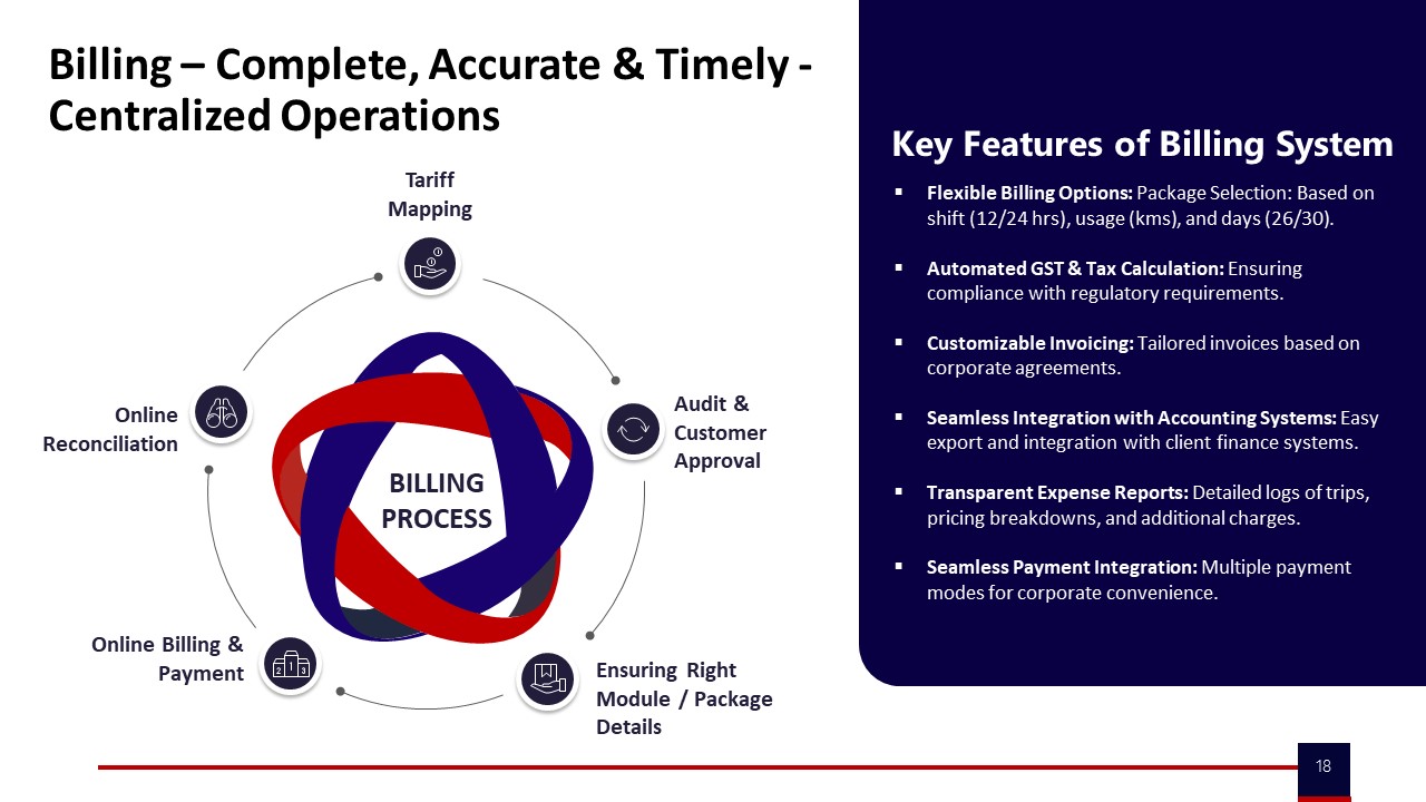
For duplicate billing, leakage is controlled by centralized, automated billing systems that map tariffs to verified trip data. Collateral on centralized billing and “Billing – Complete, Accurate & Timely – Centralized Operations” demonstrates how tariff mapping, online reconciliation, and customer approvals ensure that only one invoice is generated per verified trip or duty slip. Integration of trip logs, GPS data, and client approvals into a single billing workflow significantly reduces manual entry and duplicate submissions.
To prevent these controls from slowing down night-shift dispatch, organizations keep validations mostly automated and back-loaded. The dispatcher and driver work off pre-validated rosters and routes generated by the EMS platform, with routing and manifest sync handled by the routing engine and driver app stack. The command center operates as an always-on safety net, using real-time dashboards and alerts (geofence violation, device tampering, SOS) to intervene only on exceptions rather than every trip. Manual overrides are allowed under defined SOPs, with all overrides logged for next-day review, so operations can move quickly at 2 a.m. while Finance, HR, and Security still receive complete, audit-ready records linked to centralized dashboards and billing systems.
How should leadership set the right balance between cutting dead miles and keeping buffer capacity for disruption days, so Ops isn’t blamed when things go sideways?
B0306 Set dead-mile vs buffer trade-offs — In India shift-based employee transport (EMS), how should senior leadership decide the acceptable trade-off between minimizing dead miles and maintaining buffer capacity for disruption days, so Operations isn’t blamed when reality breaks the model?
In shift-based employee transport in India, senior leadership should define dead-mile minimization and buffer capacity as an explicit, policy-level trade-off tied to uptime and risk, not as an ad-hoc operational fight on bad days. Leadership should set target bands for dead mileage and minimum standby capacity, backed by clear SLAs, exception rules, and business-continuity triggers, so Operations executes within guardrails instead of absorbing blame when disruptions hit.
Leadership decisions work best when anchored to reliability outcomes, not only cost. On-time performance, trip adherence, and fleet uptime are the primary “non-negotiables” in EMS, because they protect attendance, productivity, and safety. Dead mileage reduction improves unit economics and carbon intensity, but aggressive cuts increase exposure to driver shortages, weather, traffic, and political events. A common failure mode is procurement or finance pushing for near-zero idle capacity without aligning with business continuity plans, which later forces Transport Heads into constant firefighting and erodes trust.
A practical approach is to codify the trade-off as part of the Target Operating Model and BCP. Leadership can mandate a baseline buffer fleet or standby capacity by timeband and site, define when additional capacity can be activated under disruption scenarios, and link these rules to vendor SLAs and commercial models. Outcome-based contracts can then reward reduced dead mileage under normal conditions while protecting minimum standby and rapid scale-up rights under defined disruption triggers, with evidence coming from command-center telemetry and incident logs. This structure reduces ambiguity, keeps Operations within a defensible envelope, and makes deviations auditable rather than personal.
- Define OTP and uptime targets first, then derive acceptable dead-mile and buffer bands from them.
- Lock disruption-day playbooks into BCP with clear triggers and pre-approved extra capacity.
- Align Finance, Procurement, HR, and Transport on these bands so cost savings never silently override continuity.
- Use command-center data to review dead mile vs. buffer performance periodically and adjust bands transparently.
What’s the minimum weekly/monthly reporting pack Finance should get for CET/CPK, seat-fill, dead miles, and productivity signals—without dashboard overload?
B0307 Minimum reporting pack without overload — In India enterprise employee mobility (EMS), what “minimum viable” reporting pack should a Finance Controller expect weekly and monthly to track CET/CPK, seat-fill, dead miles, and productivity proxies without drowning the team in dashboards?
A Finance Controller in India’s EMS context should insist on a very small, standard “control pack” that fixes definitions and trends for CET/CPK, seat-fill, dead mileage, and basic productivity proxies. The reporting pack should be simple enough to review in 10–15 minutes, but stable and auditable across months.
A weekly pack works best as an operational early-warning layer. The weekly view should focus on directional movement and exceptions instead of full financial reconciliation. A concise one-pager usually suffices if it contains a single CET and CPK view, seat-fill versus target, dead mileage percentage, and on‑time performance as a proxy for productivity and potential hidden cost. Weekly trends help Finance see where leakages or cost drifts are forming before they appear in the monthly books.
A monthly pack should be the “source of truth” that reconciles with billing and can be used in audits. The monthly view should lock the exact CET and CPK baselines, show average and 90th percentile values for seat-fill and dead mileage, and link these to contractual SLAs and outcome clauses. It should also summarize exception buckets such as no‑shows, ad‑hoc trips, and peak-hour buffers, because these often drive unplanned costs.
Most organizations avoid dashboard overload by defining a fixed KPI set and insisting on a single consolidated PDF or exportable summary. The core discipline is to freeze metric definitions, align them with contracts and SLAs, and treat the weekly pack as a forward-looking signal and the monthly pack as a backward-looking, reconcilable record.
- Weekly pack signals: trend lines for cost per kilometer and cost per employee trip, with week‑on‑week variance versus prior month average.
- Efficiency indicators: seat-fill percentage by main shift bands and dead mileage share of total kilometers.
- Reliability proxy: on‑time performance and no‑show rate as early indicators of productivity loss and potential future escalation.
- Monthly pack controls: reconciled CET/CPK by site and vendor, audit-ready trip and kilometer totals, and a short variance explanation section that ties operational deviations to cost impact.
Post go-live, how can our Transport/Facilities manager prove toil has actually reduced (fewer exceptions and reconciliations), not just shifted to new spreadsheets?
B0308 Prove toil reduction post go-live — In India corporate Employee Mobility Services (EMS), after implementation, how can a Transport/Facilities manager prove that fewer manual exceptions and reconciliations are happening (a real reduction in toil), rather than the same work being hidden in different spreadsheets?
A transport or facilities manager can prove that manual exceptions and reconciliations have genuinely reduced only when the new EMS setup produces auditable, time‑stamped evidence of work done in the command center, not just cleaner summary reports from Excel. The proof relies on operational telemetry from the EMS platform and NOC tools that explicitly track exceptions, handling time, and how many trips bypass automated flows.
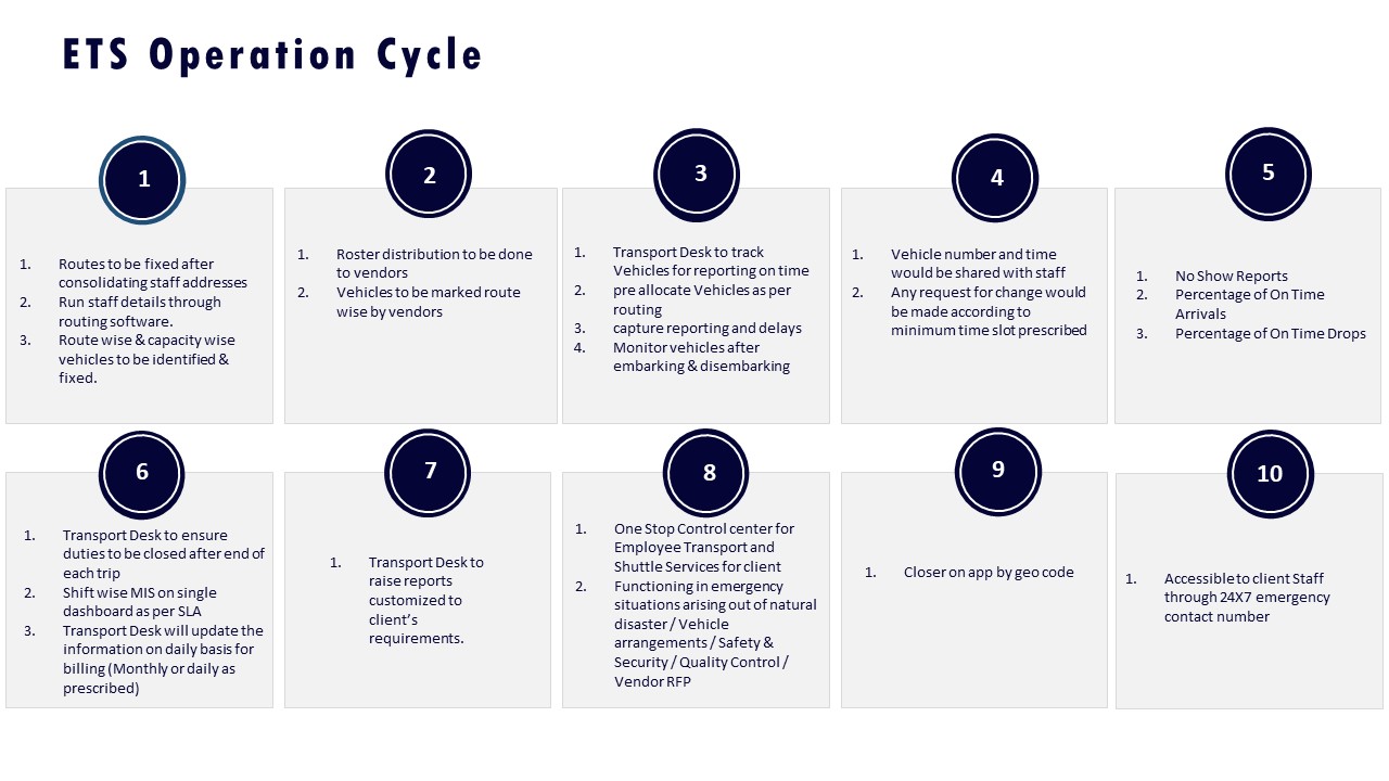
First, organizations need exception and closure metrics built into the EMS operation cycle. The ETS Operation Cycle and Dashboard – Single Window System collateral show how trip deviations, no‑shows, delays, and service reports can be captured as structured events rather than ad‑hoc calls or emails. When exception logging moves into the platform, the manager can track the count of exceptions per 1,000 trips and the mean time from detection to closure, and then show a downward trend over months.
Second, the manager should use data from the Command Centre and Transport Command Centre dashboards to demonstrate that dispatch, routing, and compliance checks are flowing through automated modules. When routing, rostering, vehicle assignment, and safety checks are handled through systems like Commutr and the Admin Transportation App, the platform can expose ratios such as “auto‑routed vs manually edited trips” or “auto‑approved vs manual override bookings.” A rising share of system-handled trips is direct evidence that manual interventions are shrinking in the live operation, not just in the final MIS.
Third, reconciliation effort must be measured explicitly. The Billing – Complete, Accurate & Timely and Billing features collaterals describe centralized, automated tariff mapping, online reconciliation, and integrated accounting. A manager can track the number of billing disputes raised per cycle, the volume of manual credit notes, and the average age of open reconciliation tickets. A meaningful reduction in disputed invoices, manual adjustments, or off‑system corrections per billing cycle indicates less hidden toil versus legacy spreadsheet reconciliations.
To ensure toil is not simply displaced, organizations should set three or four simple control KPIs and review them in monthly governance with HR and Finance:
- Exceptions per 1,000 trips and their closure SLA, based on NOC and alert supervision logs.
- Share of trips fully processed via the EMS platform (booking → routing → tracking → billing) without manual override, drawn from tools like Commutr and the Transport Command Centre.
- Billing discrepancies and reconciliation tickets per cycle, using centralized billing system reports.
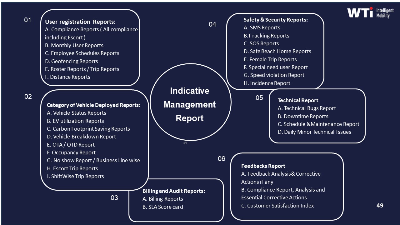
- Manual spreadsheet-based reports still in use, identified through the Indicative Management Report and phased out over time.
When these metrics are generated directly from the EMS and command center systems and show sustained improvement, the transport or facilities manager can credibly demonstrate to Finance and HR that manual firefighting, shadow spreadsheets, and ad-hoc reconciliations have actually reduced, rather than being pushed out of sight.
In the first 60–90 days, what checks should our CFO run to ensure seat-fill gains are real and sustainable, not from restricting requests or shifting costs into exceptions?
B0309 90-day checks for sustainable seat-fill gains — In India EMS shift transport, what post-purchase checks should a CFO run in the first 60–90 days to confirm seat-fill improvements are sustained and not achieved by temporarily restricting requests or pushing costs into exceptions?
In Indian EMS shift transport, a CFO should validate seat-fill improvements in the first 60–90 days by tying them to underlying trip and cost data, not just headline utilization KPIs. The core principle is to reconcile seat-fill gains with stable or improved access for employees and transparent treatment of all trips, including exceptions and ad-hoc movements.
In practice, sustainable seat-fill improvement shows up as higher Trip Fill Ratio with flat or lower no-show rates, stable or reduced exception trips, and no unexplained spikes in “off-contract” or manual-billed movement. A common failure mode is vendors inflating utilization by capping bookings, denying low-demand routes, or shifting trips to non-EMS channels that bypass the main contract.
Key checks a CFO should run in the first 60–90 days include:
- Compare pre‑ and post‑go‑live employee trip counts per shift and per site and check that total served employees have not dropped in parallel with seat‑fill gains.
- Track no‑show and “request rejected / not routed” rates by week to detect hidden rationing or silent capping of low‑density routes.
- Analyze the share of trips tagged as “exception / ad‑hoc / manual” and reconcile their cost to invoices to ensure volume is not being pushed outside the EMS platform.
- Reconcile trip‑ledger data to billing lines to confirm that every billed kilometer and trip ID maps back to a governed route with clear seat‑fill and OTP metrics.
- Review per‑employee trip cost (CET) and cost per kilometer (CPK) trends to confirm that utilization gains are not offset by higher exception tariffs or shadow vendors.
- Segment seat‑fill and access metrics by time band and gender to ensure women’s night‑shift routing has not been restricted to boost averages.
- Check that HRMS‑linked roster volumes and actual transported headcount align, which reduces the risk of suppressed demand or forced mode shift.
- Ask for independent route adherence and random route audit samples to validate that “optimized pooling” has not degraded travel time or safety patterns.
These checks should be formalized into an early post‑implementation review with Transport, HR, and Procurement so that commercial incentives continue to reward genuine efficiency rather than hidden denial of service.
cost integrity & productivity linkage
Translate CET/CPK, seat-fill, and dead-mile into measurable productivity and attendance outcomes, with auditable savings and guardrails against gaming.
How do we handle the HR vs Finance conflict when HR wants convenience but Finance is pushing seat-fill targets and dead-mile caps for EBITDA?
B0310 Resolve HR convenience vs Finance efficiency — In India corporate employee transport (EMS), how do you handle stakeholder conflict when HR prioritizes employee convenience but Finance is pushing hard for seat-fill targets and dead-mile caps tied to EBITDA goals?
In India EMS programs, stakeholder conflict between HR’s employee convenience focus and Finance’s seat-fill and dead-mile targets is best handled by making reliability and safety non-negotiable, and then optimizing cost within clearly defined service guardrails. The transport head can operationalize this by agreeing shared rules of the game, instrumenting data for both comfort and cost KPIs, and using the command center to run controlled experiments rather than opinion-based fights.
A common failure mode is starting with blanket seat-fill targets and aggressive dead-mile caps without shift-windowing and policy tiers. This often breaks OTP, increases complaints, and pushes HR into defensive mode. A more stable pattern is to segment routes and personas first. High-risk bands like women’s night shifts and critical production roles should get lower pooling thresholds and more direct routing. Less sensitive day-shift corridors and high-density tech parks can carry stricter seat-fill expectations and tighter dead-mile controls.
Command-center data and EMS tooling are crucial to de-personalize disagreements. Real trip logs, OTP%, Trip Fill Ratio, dead mileage, and complaint data let teams prove where aggressive pooling starts to erode reliability or safety. Short pilots with clear baselines help. For example, increasing pooling on two day-shift corridors for four weeks while tracking CET, OTP%, and complaints gives Finance real EBITDA-linked savings, and gives HR evidence-backed red lines.
A practical SOP is to agree a small KPI matrix up front. HR owns CEI or commute-NPS and incident rate thresholds. Finance owns CET and dead-mile caps. Transport owns OTP% and Trip Adherence Rate. When a proposed cost measure pushes any safety or experience KPI outside its band, the change is either rolled back or redesigned, rather than argued anecdotally.
images:
What vendor behaviors usually cause dead-mile creep (bad positioning, weak shift handoffs, late driver login), and how do we control it without constant manual supervision?
B0311 Vendor behaviors that drive dead-mile creep — In India corporate EMS, what specific operational behaviors by vendors usually cause dead-mile creep (poor vehicle positioning, weak shift handoffs, late driver login), and how do you build controls that don’t rely on heroic manual supervision?
In India corporate EMS, dead-mile creep is usually driven by three vendor behaviors. Vendors position vehicles reactively instead of by shift-window patterns. Vendors run weak shift handovers with no enforced cut-off or overlap logic. Vendors allow undisciplined driver app usage, so “online” time, location, and availability are not trustworthy.
Vendors cause dead mileage when fleet deployment is ad-hoc. Vehicles roam or park near driver homes instead of near high-density pick-up clusters. Route planning is done manually or late, so first and last legs become long empty runs. Fleet tagging by timeband and zone is missing, so sedans and shuttles are not anchored to specific shifts or hubs.
Dead-mile creep also comes from poor shift handoffs. Outbound and inbound shifts are planned in isolation. There is no enforced rule that vehicles finishing a drop must be positioned for the next shift window. Late roster finalization and last-minute roster edits force vehicles to start far from the first pick-up point.
Driver behavior amplifies these issues. Drivers log into the app from home or distant locations. Breaks and refuelling are unstructured, causing empty repositioning between trips. GPS tampering or intermittent connectivity hides actual dead runs and weakens audit trails.
Controls that avoid heroic manual supervision are technology- plus policy-led. Organizations define shift windowing, zone allocation, and dead-mile caps as explicit routing-engine constraints, not as “best efforts.” Command centers use a Vehicle Utilization Index and Trip Fill Ratio to flag patterns where empty kilometers are rising against fixed baselines.
Effective setups link driver app login to geo-fenced zones and timebands. Drivers can only start duty within defined hubs and windows. Dynamic routing engines are configured to minimize first-leg and last-leg distance as a core optimization parameter. Exception dashboards highlight repeated out-of-zone starts and long empty legs for vendor-level review.
Procurement and commercial models embed dead-mile controls. Contracts define caps for dead mileage per shift or per route, with penalties when breached. Fleet mix policies (sedan/MUV/shuttle/EV) are codified to prevent structural overkill on low-demand routes. Vendor tiering and rebalancing rules are tied to sustained performance on utilization, not just raw OTP.
Command-center operations run as continuous assurance instead of manual heroics. Alerts trigger when OTP is fine but CET and dead mileage trend up, indicating hidden inefficiency. Random route adherence audits validate that vehicles follow optimized dispatch, not driver-preferred routes. Driver fatigue metrics are monitored to ensure that repositioning is not a by-product of informal trip swapping.
What’s a quick, credible way to estimate the cost impact of attendance instability caused by unreliable transport, so HR can justify fixes without overstating it?
B0312 Quick estimate of attendance instability exposure — In India shift-based employee mobility (EMS), what’s the quickest way to estimate the financial exposure from poor attendance stability caused by commute unreliability, so a senior HR leader can justify investment without overstating the case?
The quickest way for a senior HR leader to estimate financial exposure from commute‑driven attendance instability is to translate late logins and no‑shows into a simple “cost per lost productive hour” model, using just three inputs: affected headcount, frequency of commute issues, and an average fully‑loaded cost per employee hour. This produces a conservative, defensible number that links transport reliability directly to payroll waste and shift output without needing complex analytics.
HR leaders can start from what is already visible in EMS operations. Most EMS programs track on‑time performance, no‑show rate, and complaint volumes through command‑center dashboards, trip logs, and HRMS attendance. Commute unreliability usually appears as repeated late logins, extended grace periods, or idle time when teams wait for delayed colleagues, and these patterns can be approximated even if data is fragmented. A small sample window, such as two representative weeks with shift‑wise variance, is usually enough to get realistic averages.
The exposure estimate becomes credible when framed as a narrow, conservative slice of the true impact. Many organizations only count confirmed commute‑linked late arrivals and complete absences, exclude borderline cases, and cap the assumed lost time per incident to one hour or less. This avoids overstating soft impacts like morale or long‑term attrition, while still showing that even a modest commute failure rate across large shift‑based workforces translates into meaningful recurring cost. That framing helps HR justify EMS improvements—such as higher SLA expectations, better routing, or command‑center investments—without triggering skepticism from Finance or Procurement.
In vendor selection, what should Procurement ask to confirm their festival/weather/Tier-2 sensitivity analysis is real and ops-grounded, not generic?
B0313 Validate realism of vendor sensitivity analysis — In India corporate EMS, during vendor selection, what questions should Procurement ask to validate that the bidder’s sensitivity analysis for festivals, weather disruptions, and Tier-2 constraints is grounded in real operations rather than generic assumptions?
In India corporate EMS procurement, the most useful validation questions force bidders to expose their data sources, historical playbooks, and command-center practices for disruptions, rather than describing “smart routing” in abstract terms. Procurement teams should ask questions that separate documented, repeatable SOPs from generic claims about traffic or weather.
A first line of questioning should probe evidence of past disruption handling. Procurement should ask for specific case studies where the bidder maintained on-time performance during monsoon, political strikes, or major festivals, including the baseline OTP, the achieved OTP, and quantified impact on customer satisfaction or complaints. Procurement should request details on how routing and capacity plans changed for those events, how quickly changes were executed, and what governance mechanism or command center monitored exceptions and escalations.
Next, Procurement should test the bidder’s sensitivity modeling for Tier‑2 and Tier‑3 cities. Questions should focus on how the bidder models constraints like driver availability, limited charging or fuel infrastructure, and local permit or compliance nuances in these locations. Procurement should ask what data inputs feed these models, such as historical trip adherence, dead mileage, and vehicle utilization patterns in specific Tier‑2 corridors. It is also useful to ask how the bidder adjusts commercial models, buffers, and fleet mix policies for Tier‑2 environments where supply is thinner and disruption risk is higher.
Procurement should also validate whether disruption assumptions are integrated into the bidder’s routing and command-center operations. Questions should cover how real-time analytics, dynamic route recalibration, and traffic trend analysis are used to predict festival traffic or weather delays, and how far in advance capacity buffers are planned. It is important to ask who in the bidder’s organization is accountable for continuous monitoring of such risks, what KPIs they track during disruption windows, and how those KPIs are reported to clients through dashboards or management reports.
Targeted questions that often surface whether the bidder is grounded in operations include:
- “Show one week of actual ETS or EMS routing and OTP reports from a peak festival period and explain the changes versus a normal week.”
- “For a Tier‑2 city of our choice, describe your current supply footprint, average vehicle utilization index, and dead mileage trends, and how these shape your proposed buffers.”
- “Walk through the step-by-step business continuity and escalation workflow in your command center when heavy rain or a bandh is announced mid-shift.”
- “Which KPIs do you actively monitor during disruptions, and how do these KPIs feed into penalties, incentives, or route corrections in near real time?”
These kinds of questions compel bidders to reveal whether they operate with a defined business continuity plan, a structured command-center model, and data-driven insights, or whether they are extrapolating from generic assumptions about traffic and weather without operational depth.
What metrics and story should Ops use to show leadership we have control—efficient CET/CPK, stable seat-fill, and predictable attendance—without it sounding like excuses?
B0314 Ops narrative for operational mastery — In India corporate employee transport (EMS), what metrics and narratives help an Operations leader demonstrate “operational mastery” to executives—showing cost efficiency (CET/CPK), stable seat-fill, and predictable attendance outcomes without sounding like excuses?
In India EMS operations, an Operations / Transport Head demonstrates “operational mastery” by consistently showing a small, stable set of metrics that tie directly to shift stability, attendance, and cost, and by presenting every deviation with a clear root cause and corrective action, not a story about traffic or vendors.
Executives respond well when Operations leads with on-time performance, cost per employee trip, and seat-fill, and then links these to attendance and incident-free shifts. This framing converts daily firefighting into a controlled, measurable system instead of a sequence of excuses.
For EMS in particular, three metric clusters usually signal control.
- Reliability & predictability. On-Time Performance for pickups and drops by shift window. Trip Adherence Rate and exception-closure time from alert to resolution. Stable OTP at or above an agreed threshold (for example, 97–98%) shows that delays are rare and managed.
- Cost & utilization. Cost per Kilometer and Cost per Employee Trip trended by month. Trip Fill Ratio and dead mileage share on pooled routes. Showing CET/CPK holding or improving while OTP and safety stay stable proves that efficiency is not coming at the expense of reliability.
- People & outcomes. Commute Experience Index or transport NPS. Complaint volume and closure SLA. Simple attendance deltas for transport-dependent shifts. Linking “high OTP + high seat-fill” to “fewer late logins and fewer escalations” turns raw fleet data into a business outcome story.
An Operations leader who wants to avoid sounding defensive usually presents each review in a repeatable pattern. The pattern focuses on what was controlled, what changed, and how quickly issues were closed, instead of why they happened.
- Start with a one-page dashboard of 6–8 KPIs across reliability, cost, safety/compliance, and experience. Keep definitions constant across months.
- Highlight two or three “wins” where routing, command-center alerts, or driver management prevented problems or absorbed disruptions. This shows early-warning capability, not just post-facto reporting.
- For any dip in OTP, CET, or seat-fill, provide a quantified impact, a root-cause category, and a specific corrective SOP. Executives tend to accept “we changed the rule or process” more than “there was rain and traffic.”
- Show how centralized command-centre monitoring, alert supervision, and daily shift briefings reduced manual firefighting. For example, fewer emergency reallocations, reduced no-shows, and faster incident acknowledgment.
Narratives that earn trust are short and repeatable. Strong examples include “We held CET flat while improving fleet uptime and seat-fill,” “We maintained women-safety and compliance with zero major incidents and full audit trails,” and “We used real-time routing and command-center alerts to keep OTP above target through weather and infrastructure issues.” Each of these statements ties the metric to an operational control rather than to luck.
How can our CFO link CET/CPK savings to real productivity and attendance gains in our employee commute program, using data we can trust?
B0315 Proving cost-to-productivity linkage — In India-based Employee Mobility Services (EMS) for enterprise employee commute programs, how can a CFO credibly link cost per employee trip (CET) and cost per kilometer (CPK) improvements to measurable productivity and attendance stability outcomes, without relying on vendor-reported numbers?
In India-based Employee Mobility Services, a CFO can link CET/CPK improvements to productivity and attendance stability only by building an internal, cross-system data model that ties verified trip data to HR attendance, login times, and shift adherence, instead of relying on vendor summaries. The core principle is to treat vendor feeds as raw telemetry, then reconcile and analyze them inside the enterprise data estate, using HRMS, finance, and access-control systems as the “source of truth” for outcomes.
The CFO’s team can first standardize CET and CPK definitions across all EMS contracts. Finance teams can normalize costs for dead mileage, empty legs, night premiums, and taxes, then compute CET and CPK directly from invoices, tariff tables, and approved trip counts. This reduces dependence on vendor-claimed savings and makes per-trip economics auditable.
Productivity and attendance impact can be measured by correlating EMS data with HRMS and operations metrics. HRMS timestamps for swipe-ins, system logins, and shift adherence can be mapped to verified trip manifests, on-time performance, and exception logs stored in a mobility data lake. Higher on-time pickups often align with fewer late logins and reduced productivity noise, which HR can quantify as a drop in manager complaints or adherence breaches.
A CFO can then define a small, fixed KPI set for internal dashboards. Typical signals include CET trend versus attendance volatility, CPK versus overtime or shrinkage in specific shifts, and no-show or cancellation rates versus SLA breaches and exception closure times. These indicators can be calculated from reconciled HRMS, ERP, and command-center logs, which gives Finance defensible narratives for auditors and the board.
To keep this credible, organizations can adopt a few operating rules. They can mandate vendor data portability and consistent schemas in contracts, run periodic route adherence and trip audit samples, and insist that all outcome claims be reproducible from enterprise-side systems. They can also apply simple anomaly detection checks, such as flagging routes with high CPK but no corresponding reliability benefit, or sites where CET drops but late-login penalties or shrinkage rise.
How can HR figure out if OTP issues are truly causing attendance problems (not just getting blamed), and what proof should we capture?
B0316 Diagnosing OTP vs attendance impact — In India corporate employee transport operations (EMS), what are practical ways an HR leader can diagnose whether poor on-time performance (OTP) is actually driving attendance volatility versus managers simply blaming transport, and what evidence should HR collect to prove causality?
An HR leader can diagnose whether poor on-time performance is truly driving attendance volatility by directly correlating trip-level OTP data with attendance logs, shift compliance, and complaint patterns over time. HR should build simple, auditable comparisons that show whether no-shows, late logins, and attrition are higher on routes, shifts, or days where employee mobility services underperform versus where OTP is stable.
First, HR should obtain structured OTP data from the transport command center or vendor. The data should include trip IDs, scheduled vs actual pickup/drop times, routes, vehicles, drivers, and exception flags such as “cab no-show” or “driver late.” A centralized command centre with real-time monitoring and alert supervision systems will typically already track OTP%, geofence violations, and over-speeding, and this same data can evidence operational reliability by route and shift.
Next, HR should align this with HRMS attendance and productivity data. HR should compare late login patterns, early logouts, and no-shows against the exact employees and shifts that used corporate transport. A practical method is to segment employees into “using EMS” and “not using EMS” for the same process and timeband. HR can then compare late login rates and absence volatility between the two cohorts. If transport is the real driver, late attendance should spike specifically where OTP and route adherence scores are weak, not across the board.
HR should also examine complaint and feedback channels. Commute feedback from employee apps and safety/incident logs from the command centre can be tagged by route, vendor, and shift. HR should look for clusters where repeated OTP complaints co-exist with localised attendance problems. In contrast, if managers broadly “blame transport” but the command centre shows 98% on-time arrival in that corridor, HR gains evidence that performance issues lie elsewhere.
To prove a causal link, HR should run simple before–after or A/B style checks. For example, where the transport team has implemented dynamic route optimization during monsoon conditions and achieved a 98% on-time arrival rate with a 10% increase in customer satisfaction, HR can check whether late login complaints and manager escalations from those same teams reduced in the following month. Similarly, when a problematic route or vendor is replaced, HR can track whether attendance volatility on that route normalizes.
The most persuasive evidence pack for leadership usually contains three elements. The first is a time series chart showing OTP% and late login% for the same employee cohort across several weeks, highlighting correlated peaks and drops. The second is a route-wise or shift-band comparison table showing that the worst OTP routes also have the worst attendance volatility, while well-performing routes do not. The third is a cluster of anonymised employee feedback quotes and ticket logs that explicitly mention missed cabs, long delays, or safety concerns, timestamped and matched to specific low-OTP trips.
A common failure mode is relying on isolated anecdotal incidents or vendor assurances without tying them back to measurable KPIs. HR should insist on audit-ready logs from the transport provider’s dashboards, including trip adherence reports, deviation reports, and exception closure SLAs, and then map these to HR’s absence and grievance records. If managers’ claims are valid, HR will see systematic patterns where poor OTP precedes spikes in absenteeism or productivity dips. If not, HR can confidently redirect the conversation toward performance management, having demonstrated that mobility operations are stable and auditable.
How do we set seat-fill and dead-mile targets in a way that helps dispatch daily without increasing missed pickups and night escalations?
B0317 Seat-fill targets without escalation — In India enterprise-managed Employee Mobility Services (EMS), how should an operations or facility transport head translate seat-fill ratio targets and dead-mile caps into day-to-day dispatch decisions without creating missed pickups or 3 a.m. escalations?
In India EMS operations, a transport or facility head should treat seat-fill targets and dead-mile caps as guardrails applied through SOPs and routing rules, not as hard quotas applied trip-by-trip. Dispatch decisions should prioritize guaranteed pickups and OTP, while continuously nudging routing, fleet mix, and vendor usage toward target seat-fill and dead-mile levels over each shift and week.
Daily firefighting usually starts when economic targets override operational buffers. A common failure mode is pushing for very high seat-fill on every route and cutting standby capacity. This approach often increases no-shows, delays, and 3 a.m. escalations, especially under hybrid attendance and traffic variability. Most organizations stabilize EMS when they lock a minimum reliability baseline first, then optimize within that guardrail using routing tools, command-center monitoring, and vendor governance.
Practically, a transport head can convert the commercial targets into dispatch rules and checks such as: - Defining shift-wise “green bands” for seat-fill. For example, 75–85% for peak shifts and slightly lower for late-night or high-risk corridors, instead of demanding 95–100% on every cab. This keeps room for last-minute adds and avoids routing employees into unsafe or excessively long detours. - Setting dead-mile caps at the route and shift level, not per vehicle. For example, cap total dead mileage per shift window and per depot, and let the routing engine minimize it subject to OTP and maximum ride-time constraints. - Encoding non-negotiable safety and experience constraints in routing logic. For instance, maximum time-in-cab, women-first night routing, escort rules, and geo-fence exclusions must not be traded off to chase a marginally better seat-fill ratio.
The command center plays a critical role in converting these rules into early alerts instead of late surprises. Real-time dashboards and alerts can track live seat-fill, dead mileage, and route adherence. Exception flags such as repeated under-filled circuits, high dead runs from a particular hub, or specific vendors causing excess repositioning help operations teams adjust rosters or vendor allocation for the next shift instead of over-optimizing the current one.
To avoid 3 a.m. escalations, operations teams benefit from: - A small, policy-backed buffer of vehicles during sensitive timebands and on high-risk routes, funded as a known cost of reliability. Cutting this buffer to hit a short-term dead-mile target is a frequent cause of missed pickups. - A clear escalation and fallback SOP whenever app or GPS tools underperform. For example, manual call trees, SMS-based confirmations, and pre-agreed rerouting rules between the command center, vendors, and drivers. - Structured feedback loops from shift reports. Patterns such as recurring low seat-fill from specific pockets, or chronic dead mileage between two hubs, can inform changes in employee clustering, pickup point rationalization, or fleet mix rather than forcing dispatchers to improvise mid-shift.
Most mature EMS programs treat seat-fill and dead-mile metrics as outcome KPIs assessed over time. Dispatchers are guided by routing rules, buffers, and early alerts that prevent missed pickups, while the transport head uses analytics and vendor governance to steadily move the operation toward commercial targets without sacrificing reliability or safety.
What are the biggest leakage points that push up CET/CPK in employee transport, and what controls actually stop them in an audit-ready way?
B0318 Leakage sources and audit-grade controls — In India corporate employee commute programs (EMS), what are the most common cost leakage sources that inflate CET/CPK—such as duplicate trips, wrong distance slabs, no-show billing, detours, or manual exceptions—and what controls are considered audit-grade to prevent them?
In Indian corporate EMS programs, cost leakage usually comes from predictable operational gaps. The most common sources are inaccurate or manipulable trip data, weak linkage between SLAs and billing, and manual overrides that are not audit-traceable. Audit‑grade controls rely on end‑to‑end digital trip lifecycle management, reconciled GPS evidence, and centralized, role‑based governance rather than ad‑hoc desk decisions.
The industry brief highlights several recurring leakage patterns. Duplicate or “ghost” trips arise when bookings and completions are managed outside a unified platform and without immutable trip logs. Wrong distance or slab billing happens when tariff logic is not tightly mapped to GPS‑verified distance and duty time. No‑show and cancellation charges inflate cost per employee trip when attendance, roster, and trip manifests are not synchronized with HRMS. Dead mileage and inefficient routing increase cost per kilometre when there is no routing engine enforcing seat‑fill targets, dead‑mile caps, and dynamic route recalibration. Manual exceptions, such as off‑platform extensions or vehicle upgrades, leak cost when they bypass approval workflows and are not tagged with reason codes.
Audit‑grade prevention relies on a few hard controls. Centralized, technology‑driven trip lifecycle management is considered foundational because it ensures every trip has a single source of truth from booking to billing, including OTP-based boarding, GPS tracks, and automated closure. GPS‑anchored billing, where distance, duration, and route adherence are pulled from tamper‑evident telematics, limits disputes over slabs, detours, and idle time. Tight HRMS and roster integration closes gaps between who was scheduled, who actually travelled, and what was invoiced. This reduces bogus no‑shows and duplicate trips and ties CET directly to real attendance.
Vendor and tariff governance are also critical. Clear service catalogs and tariff mapping by persona, route type, and timeband reduce ad‑hoc usage of higher‑cost models. Outcome‑linked contracts, where payouts are indexed to OTP, seat‑fill, and SLA compliance, create economic disincentives for inefficient routing and under‑utilized vehicles. Centralized billing systems with automated tax calculation, tariff mapping, and online reconciliation, as shown in the billing collaterals, are often used to make invoices traceable to raw trip data and MIS.
Command‑center‑driven observability strengthens these financial controls. A 24x7 NOC or command center monitors route adherence, exceptions, and incident closure times in real time. This setup supports early alerts when detours, repeated manual overrides, or abnormal patterns emerge in specific routes, timebands, or vendors. When combined with data‑driven insights dashboards that expose cost, utilization, and SLA KPIs, transport heads can systematically reduce dead mileage and enforce routing standards rather than firefighting individual escalations.
For an EMS operator focused on daily reliability, the practical control set usually includes: enforcing platform‑only bookings and dispatch; GPS‑based distance and time capture mapped directly to tariff slabs; mandatory OTP or app-based check‑in to validate boarding; restricted manual overrides with audit logs; roster–trip–invoice reconciliation at cycle close; and periodic route adherence and cost anomaly audits. These steps reduce CET and CPK without relying on after‑the‑fact negotiation, and they create the kind of evidence trail that Finance, Procurement, and auditors treat as defensible.
images:
With hybrid attendance and peak seasons like festivals/monsoons, how should Finance stress-test CET/CPK and seat-fill so we don’t get surprised later?
B0319 Hybrid and seasonal sensitivity analysis — In India Employee Mobility Services (EMS) with hybrid work and variable attendance, how should a finance controller run sensitivity analyses for CET/CPK and seat-fill when festival seasons or monsoon disruptions change shift rosters and route feasibility?
Finance controllers in India should run CET/CPK and seat‑fill sensitivity analyses by explicitly modeling 2–3 “stress scenarios” for festival seasons and monsoon disruptions, then recomputing unit economics using a small set of operational levers. Each scenario should combine attendance volatility, route feasibility changes, and EV/ICE fleet mix impacts into revised assumptions for trips, kilometers, and usable seats.
The starting point is a clean baseline under normal conditions. Finance teams should work with the transport head and HR to lock one reference month with stable hybrid rosters, documented route plans, and typical OTP/seat‑fill performance. That baseline should define current Cost per Employee Trip (CET), Cost per Kilometer (CPK), Trip Fill Ratio (seat‑fill), dead mileage, and EV utilization ratio for each shift band.
For festival periods, finance controllers should define scenarios with lower attendance and higher no‑show rates. Each scenario should adjust seat‑fill, number of routes, and duty cycles to reflect more empty seats and potential shift consolidations. CET should then be recomputed under three patterns. One pattern is “keep capacity constant,” which stabilizes OTP but increases CET and CPK since dead mileage rises. Another pattern is “aggressively consolidate,” which lowers CET but may worsen employee experience and OTP. A third pattern is “hybrid,” which uses flexible models like per‑seat or trip‑based pricing on marginal routes while retaining fixed models where volume is stable.
For monsoon and weather disruptions, sensitivity analysis should introduce parameters for extended trip times and rerouting. Finance should model longer average kilometers per trip, increased buffer vehicles, and temporary drops in fleet utilization index. CPK will rise due to extra distance and idle time. CET may also increase if SLA clauses allow surge or standby charges. Finance controllers should work with the command center and routing team to estimate a “rain‑day profile,” using past monsoon case studies where dynamic route recalibration still maintained on‑time arrivals with increased operational effort.
EV fleets require a separate layer of sensitivity. Monsoon and festival patterns can change ideal charging windows and shift feasible routes between EV and diesel. Finance should model EV utilization ratio and charger access under each scenario. In some cases, EVs preserve CET by lower running cost even when utilization dips. In others, limited charging infrastructure or range risk can force more ICE deployment, raising CPK and emissions. The EV‑shift impact should be reflected as a delta in CET, CPK, and gCO₂ per passenger‑kilometer.
To keep the analysis operationally grounded, finance controllers should build the model around a few controllable levers. These levers include fleet size per timeband, backup fleet buffers, operating models (per‑km vs per‑trip vs per‑seat), and routing policies such as maximum detour limits and acceptable seat‑fill thresholds. Each lever changes CPK and CET differently. For example, higher buffer fleets improve resilience but increase cost per kilometer, while strict seat‑fill targets lower CET but risk late arrivals during monsoon congestion.
A practical way to structure the work is to define three tiers of scenarios. The first tier is “mild variation,” where attendance shifts ±10% and travel time increases moderately during early or late monsoon days. The second tier is “severe but planned,” such as major festivals where a large proportion of employees are on leave and routes can be pre‑consolidated. The third tier is “severe and unplanned,” such as flooded corridors or sudden route closures that require full reliance on business continuity plans and dynamic fleet reallocation.
Within each tier, finance controllers should request from operations a simple sensitivity table. The table should map seat‑fill, dead mileage limits, and OTP targets to expected CET and CPK. This table should also highlight which commercial models (monthly rentals, per‑km, pay‑per‑usage) are most resilient at that level of volatility. For example, a monthly rental model may be efficient at high, stable utilization, but a pay‑per‑usage model could be cheaper when festival attendance is very low.
A key success factor is consolidating the outputs into a single management dashboard. The dashboard should show, for each scenario, the impact on total monthly spend, unit economics, OTP, and incident risk. It should also indicate how much of the cost change comes from temporary measures like backup fleets and rerouting. This allows finance, HR, and transport to agree ahead of time which combination of cost and reliability they will accept during these periods.
images:
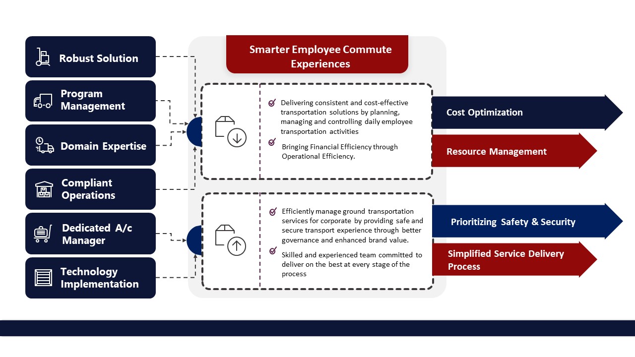
For Tier-2 locations, how do routing and supply constraints usually affect CET/CPK, and how should we benchmark pricing fairly vs Tier-1?
B0320 Tier-2 cost distortion and benchmarking — In India enterprise employee transport (EMS) across Tier-1 and Tier-2 cities, how do Tier-2 routing constraints (permit issues, road quality, sparse vendor supply, longer dead miles) typically distort CET/CPK, and how should procurement prevent unfair benchmarking against Tier-1 baselines?
In India enterprise employee mobility, Tier-2 city constraints usually push Cost per Employee Trip (CET) and Cost per Kilometer (CPK) above Tier-1 levels. The main drivers are structurally higher dead mileage, weaker vendor density, permit and regulatory friction, and routing through low-quality or indirect roads that depress utilization and reliability.
Tier-2 networks often require longer “empty legs” between dispersed residential clusters and industrial or IT parks. This raises dead mileage and lowers the Trip Fill Ratio, so the same rostered capacity delivers fewer billable kilometers. Sparse vendor supply restricts fleet mix optimization and limits seat-sharing, so operators lean on dedicated or semi-dedicated cabs, which improves reliability but inflates CET. Local permits, state tax tokens, and compliance overhead also add fixed cost per vehicle, which is easier to amortize in dense Tier-1 corridors than in smaller catchments.
Poorer road quality and unpredictable congestion increase duty cycles and reduce Vehicle Utilization Index. That forces higher buffer capacity and downtime allowances to maintain On-Time Performance and safety, again lifting unit costs. If procurement applies Tier-1 benchmarks without adjusting for these structural factors, vendors cross-subsidize, cut corners on safety/compliance, or eventually exit, which destabilizes Employee Mobility Services.
Procurement teams should codify a differentiated benchmark model for Tier-2. The model should:
- Break out CET/CPK by city archetype, explicitly capturing dead mileage caps, minimum fleet buffers, and seat-fill assumptions.
- Anchor evaluations on outcome KPIs (OTP%, incident rate, compliance scores) rather than raw CPK alone.
- Use transparent service catalogs and operating models (e.g., pooled vs dedicated EMS, Long-Term Rental) tailored to Tier-2 density and shift patterns.
- Embed outcome-linked commercials where penalties and incentives respect realistic Tier-2 routing and utilization envelopes.
This approach prevents unfair Tier-1 comparisons, protects safety and compliance, and gives Finance and Procurement a defensible narrative for why Tier-2 CET/CPK must sit in a different, explicitly governed band.
How do we show dead-mile reduction is improving shift adherence and productivity, not just making CPK look better on reports?
B0321 Dead-mile reduction to business outcomes — In India Employee Mobility Services (EMS), what is a defensible method to connect dead-mile reduction initiatives to business outcomes like shift adherence and productivity, rather than just reporting a lower cost per kilometer (CPK) on paper?
A defensible method is to treat dead-mile reduction as an operational intervention in routing and capacity, then link it to On-Time Performance (OTP%), Trip Adherence Rate (TAR), and seat-fill, and finally correlate those to shift adherence and attendance metrics from HRMS. Dead mileage reduction is only credible when it appears as one lever in a measurable chain from routing changes → reliability improvements → HR outcomes, not as a standalone cost-per-km story.
First, operations teams should define baselines for dead mileage, OTP%, and TAR by shift window and route cluster. Dead-mile reduction initiatives can then target fleet mix, seat-fill, and dynamic routing, with clear caps on dead mileage and peak vs non-peak buffers. A common failure mode is to chase lower CPK by cutting buffer capacity, which improves paper economics but degrades OTP and increases exception latency.
Second, organizations should integrate EMS telemetry with HRMS for time-bound pilots. Routes or sites with optimized dead mileage are tagged, and their OTP%, no-show rate, and exception-closure times are compared to control groups. Shift adherence and late-login incidents for those employee cohorts are pulled from HR systems. Dead-mile reduction is considered successful only when OTP and TAR are maintained or improved, and attendance volatility decreases.
Finally, procurement and Finance can move commercials toward outcome-linked procurement. Vendor payouts are indexed not just to kilometers billed but also to reliability KPIs such as OTP%, Trip Adherence Rate, and complaint-closure SLAs. This approach makes dead-mile initiatives accountable to both cost/TCO metrics and business outcomes like productivity, attendance, and reduced firefighting load in the command center.
What early signals can ops track to predict attendance issues from transport problems, and how do we measure them without extra spreadsheets?
B0322 Predicting attendance dips from ops signals — In India corporate ground transportation for employee commute (EMS), what early warning signals should operations monitor to predict an attendance dip caused by transport instability (driver churn, route volatility, low seat-fill, rising exceptions), and how can those signals be measured without adding manual toil?
Early warning signals for commute-linked attendance dips in India EMS are visible in transport operations days before HR sees them in login data. Operations should track a small, automated set of routing, reliability, safety, and sentiment indicators that can be fed from existing telematics, apps, and command-center logs into simple dashboards and exception alerts.
The most predictive signals sit close to daily execution. On-time performance (OTP%) should be watched by shift, route, and vendor, with thresholds for early-warning bands when OTP starts sliding even 3–5 points. Trip Adherence Rate and geo-fence violations can be monitored from GPS and IVMS, with route deviation alerts pushed into a command center rather than spreadsheets. Rising exception volume per 100 trips, including no-shows, repeated reschedules, and SOS or safety alerts, is another strong early indicator of employee frustration and eventual attendance impact.
Capacity and asset stability are the next set of signals. Operations teams can monitor Trip Fill Ratio and dead mileage from the routing engine to catch low seat-fill, which often precedes cost-cutting moves and route volatility. Driver churn, fatigue, and last-minute substitution rates can be inferred from the driver app stack and duty-cycle data, rather than from manual rosters. A spike in backup-vehicle usage, standby car deployment, or fallback to diesel in EV-heavy fleets can be logged automatically as operational instability.
To avoid manual toil, these signals should be derived from systems already in place. Streaming telematics, employee and driver apps, and the central command center can feed a mobility data lake and standardized KPI layer. Dashboards such as those used for advanced operational visibility and single-window reporting can surface OTP, Trip Fill Ratio, exception closure time, and Fleet Utilization Index with automated drill-downs. Alert supervision systems and centralized compliance management can generate rule-based notifications when thresholds are crossed, replacing ad-hoc calls and WhatsApp tracking. When combined with HRMS integration for attendance patterns and complaint closure SLAs, operations can forecast transport-driven attendance dips early enough to rebalance capacity, stabilize routes, and intervene with driver management, without adding extra manual workload.
images:
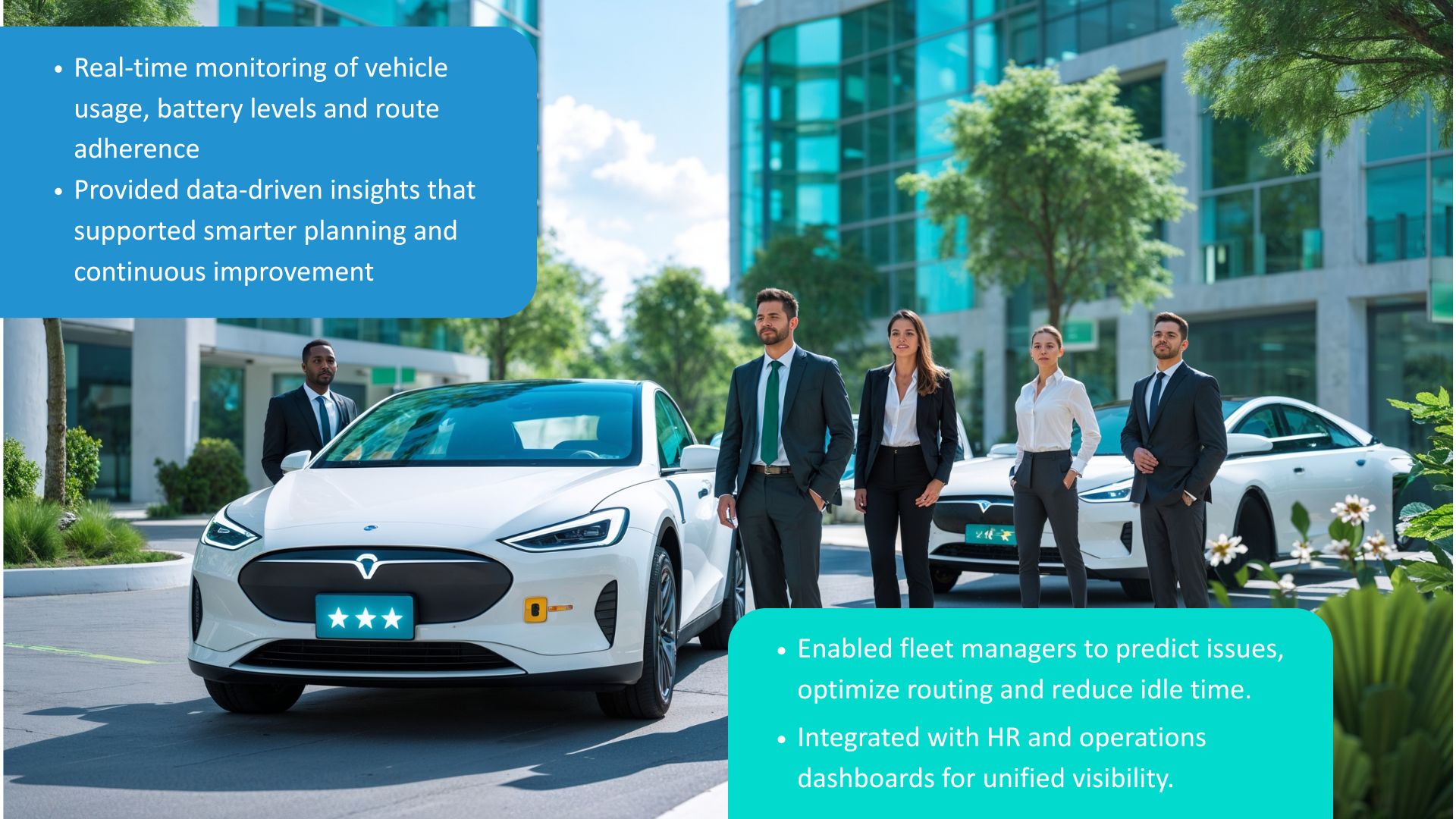
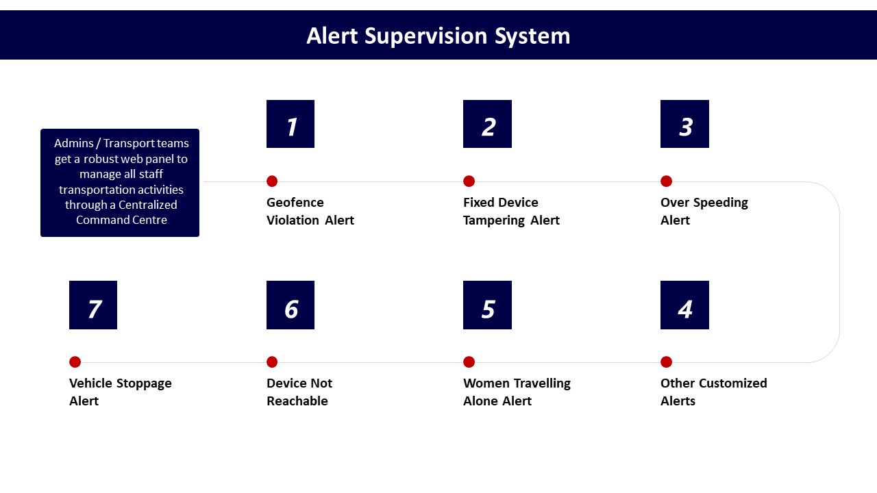
How can HR and Finance align on what ‘productivity loss from commute’ really means, so HR isn’t seen as emotional and Finance isn’t seen as just cost-cutting?
B0323 Aligning HR-Finance on productivity loss — In India EMS programs where HR owns employee experience and Finance owns spend control, how can HR and Finance agree on a shared definition of ‘productivity loss from commute’ so the CFO doesn’t dismiss HR escalation as anecdotal and HR doesn’t see Finance as cost-only?
In Indian employee mobility programs, HR and Finance align best on “productivity loss from commute” when they convert commute pain into a small, auditable KPI set that links transport reliability to attendance, shift adherence, and unit cost. A shared definition works when it uses data they both already trust, such as HRMS attendance, shift rosters, transport trip logs, and SLA metrics like OTP% and no‑show rate.
A practical approach is to anchor “productivity loss from commute” to three observable buckets. The first bucket is lost or delayed work time. HR and Finance can jointly define this as the number of late logins and missed shifts where trip logs show delayed pickup, route deviation, or vehicle no‑show. The second bucket is replacement and escalation cost. This includes overtime, backup staffing, and exception handling where poor OTP or route failures force last‑minute changes, all tagged back to specific trips and SLAs. The third bucket is avoidable transport waste. This covers repeat trips, dead mileage, and low seat‑fill that occur because of unreliable routing or fragmented vendors, which inflate cost per employee trip without adding productive hours.
The two teams can then codify these buckets in a simple, shared scorecard. HR leads on mapping commute incidents to attendance, complaints, and safety escalations. Finance leads on translating those same incidents into CET, CPK, and overtime or idle cost. Both sides agree that only commute-linked records where trip data, HRMS logs, and SLAs line up are counted. This creates a definition that is neither anecdotal nor cost-only and gives the CFO defensible numbers while giving HR a stable, evidence-backed way to escalate commute risks.
How should Procurement design commercials so seat-fill and dead-mile incentives don’t lead to unsafe pooling or longer rides that hurt attendance?
B0324 Avoiding perverse incentives in commercials — In India enterprise employee transport (EMS), how should a procurement leader structure outcome-linked commercials so seat-fill and dead-mile targets don’t incentivize unsafe pooling, longer ride times, or ‘creative routing’ that hurts attendance and productivity?
In India enterprise employee transport, procurement leaders should link commercials to a balanced KPI set that caps risk on ride time and safety while still rewarding efficient seat-fill and low dead mileage. Contracts work best when seat utilization and dead-mile reduction bonuses are conditional on hard limits for maximum ride duration, safety compliance, and on-time performance that must be met first.
Procurement should first define a narrow band for seat-fill and dead mileage. Incentives should apply only within this band. This avoids over-pooling and detours that extend routes. Seat-fill should be measured alongside a maximum ride time per shift window and route adherence audits. Vendors should earn bonuses only when all three metrics are within agreed thresholds.
Outcome-linked commercials need explicit negative incentives for “creative routing.” A contract should penalize excessive detours, repeated route changes without approval, and patterns where trips hit ride-time caps even if seat-fill looks good. OTP%, Trip Adherence Rate, and complaint trends from HRMS-linked feedback should sit alongside utilization metrics in the payment logic.
Safety and compliance must act as hard gates before any incentive is paid. Procurement should require zero-tolerance thresholds for major safety incidents, escort compliance for night shifts, and credentialing currency for drivers and vehicles. Any breach should suspend utilization-linked incentives for that period.
A practical structure uses tiered payouts with clear preconditions:
- Base payment indexed to completed trips with minimum OTP and compliance scores.
- Utilization bonus payable only if ride times, safety, and complaint SLAs are met.
- Malus triggers when extended ride times, repeated detours, or safety exceptions occur, regardless of utilization gains.
This approach keeps vendors focused on balanced outcomes. It protects HR’s attendance and safety KPIs while still giving Finance and Procurement verifiable gains on cost per trip and fleet efficiency.
images:
images:
images: 
What’s a simple way to measure toil reduction in monthly CET/CPK reconciliation, and which steps are typically the biggest time-wasters?
B0325 Quantifying toil in reconciliation — In India Employee Mobility Services (EMS), what’s a practical ‘2-click vs 10-click’ benchmark to quantify toil reduction in monthly CET/CPK reconciliation, and which process steps usually create the most avoidable operational drag?
In India Employee Mobility Services, a practical “2‑click vs 10‑click” benchmark is this. CET/CPK reconciliation is low‑toil when Finance or Transport can move from consolidated trip data to a reconciled, audit‑ready invoice view in about 2–5 focused actions inside one governed platform. It is high‑toil when the same outcome requires 10+ fragmented actions across exports, emails, sheets, and portals every month.
A 2‑click style flow usually looks like this. The transport platform already standardizes trip logs, rates, dead mileage rules, and SLAs into a single data model. Finance or Transport then only needs to 1) select period/vendor/cost center and 2) run a pre-configured reconciliation report that matches CET/CPK, utilization, and SLA outcomes to billed amounts. Any dispute drill‑down happens from the same screen without rework.
A 10‑click pattern appears when EMS data is fragmented by vendor, site, and format. Teams must repeatedly export trip files, manually normalize fields, apply tariff logic in Excel, and reconcile against opaque vendor invoices. Each exception triggers additional loops with transport desks and vendors, which increases cycle time and audit risk.
The worst avoidable operational drag typically comes from: - Manual tariff and dead‑mileage application. Teams re‑calculate slabs, waiting charges, or minimum guarantees because rules are not codified in the system. - Multi‑vendor, multi‑format trip data. Different file layouts, time formats, vehicle codes, and missing identifiers force repetitive data cleaning. - Weak linkage between SLAs and billing. OTP failures, no‑shows, or safety incidents are not auto-tagged against trips, so penalty/earnback calculations are rebuilt manually each month. - Unaligned master data across HRMS, Finance and EMS platforms. Cost centers, employee IDs, and project codes do not match, so allocations for CET and CPK require line‑by‑line corrections. - Lack of a single command‑center view. Transport heads and Finance cannot see the same governed metrics for utilization, billing, and exceptions, so reconciliation devolves into email‑driven clarification cycles.
When hybrid rosters change every day, how do we choose between better seat-fill and better OTP, and how do we explain that trade-off to leadership?
B0326 Seat-fill vs OTP trade-off narrative — In India corporate employee transport (EMS), when hybrid rosters change daily, how should operations decide whether to prioritize seat-fill optimization or on-time performance (OTP), and how can that trade-off be explained to senior leadership without losing political capital?
In Indian EMS with volatile hybrid rosters, operations should treat on-time performance as the non‑negotiable primary objective and optimize seat‑fill only within guardrails that protect OTP and safety. Seat optimization should be applied dynamically by shift window and corridor, but any routing change that risks breaching agreed OTP or safety constraints should be blocked by design.
OTP needs primacy because shift adherence, production floors, and night‑shift safety are board‑level exposures. Poor OTP creates visible business disruption for HR and line managers, while modestly lower seat‑fill mainly affects unit economics. In practice, most organizations use AI routing, dynamic route recalibration, and dead‑mileage caps to lift Trip Fill Ratio without touching critical buffers such as reporting time before shift, maximum detour minutes, or women‑safety routing rules.
The trade‑off is easier to defend with leadership when it is framed as an explicit operating policy tied to measurable outcomes. Operations teams can define three tiers. Tier 1 routes are “OTP‑first” windows and corridors where late pickups impact production or high‑risk timebands. Tier 2 routes are “balanced” where routing engines can chase higher utilization as long as observed OTP and incident metrics remain within SLA. Tier 3 use‑cases, like mid‑day non‑critical movements, can be “seat‑fill first” with aggressive pooling and dead‑mileage reduction targets.
To protect political capital, transport heads should present this as a governance decision, not a personal preference. That includes a documented policy endorsed by HR, Security, and Finance which links payout and penalties to both OTP% and utilization, with clear red lines such as minimum OTP thresholds, escort compliance, and incident‑closure SLAs. Leadership then sees that operations is not choosing between cost and reliability on the fly, but executing a board‑aligned mobility governance model under hybrid‑work volatility.
What specific data and evidence should Finance ask for so we can defend CET/CPK savings in an audit when vendors claim seat-fill/dead-mile improvements?
B0327 Audit evidence for mobility savings — In India enterprise-managed employee commute programs (EMS), what data artifacts should Finance insist on to defend CET/CPK savings in an internal audit—especially when vendors claim dead-mile reduction or higher seat-fill as the driver?
Finance should insist on a tightly linked chain of operational, financial, and governance artifacts that quantify cost per employee trip (CET) and cost per kilometer (CPK) and directly evidence dead-mile reduction and improved seat-fill.
Finance teams need trip-level operational logs that show each trip’s route, distance, timing, and occupancy, including clear separation of productive kilometers versus dead mileage. These artifacts should come from the EMS routing engine and telematics systems as exportable datasets, with immutable GPS traces, trip IDs, and timestamps that can be reconciled to vendor invoices and internal ERP records. Finance should also demand seat-fill and Trip Fill Ratio reports by route, shift window, and timeband, so higher occupancy can be shown as a measurable driver of CET improvement.
Cost defensibility in audits depends on reconciliations that tie raw trip data to billing. Finance should therefore insist on per-trip or per-roster billing back-up, tariff mapping sheets, and automated reconciliation reports that link SLAs and utilization metrics to invoiced amounts. Evidence packs should include before/after baselines for CPK, CET, dead mileage percentage, and Vehicle Utilization Index, with the calculation logic disclosed. Centralized dashboards and Indicative Management Reports are useful only when their underlying raw data, ETL logic, and aggregation rules are available for sample testing by Internal Audit.
To support claims of algorithmic optimization, Finance should ask for change-control documentation that shows when routing rules, fleet mix, or seat-fill targets were modified and how those changes correlate with shifts in CPK/CET. This should be complemented by SLA and exception reports from the command center that document route adherence, no-show rates, and variance from planned kilometers, so auditors can verify that reported savings are not coming at the expense of service quality or On-Time Performance.
- Exportable trip ledger with GPS-derived distance and occupancy, split into productive versus dead kilometers.
- Seat-fill and Trip Fill Ratio reports by route and shift, aligned with Vehicle Utilization Index.
- Tariff mapping and invoice back-up that reconcile each trip or roster to billed kilometers and rates.
- Before/after KPI baselines for CPK, CET, dead-mile %, and utilization, with transparent formulas.
- Command center SLA and exception reports linking optimization changes to reliability and OTP outcomes.
How can HR Ops quantify the real cost of unreliable commutes so Finance sees it as productivity/retention risk, not just complaints?
B0328 Turning complaints into quantified risk — In India Employee Mobility Services (EMS), how can an HR operations manager quantify the employee-side cost of unreliable commutes (complaints, drop in trust, manager escalations) in a way that Finance accepts as a productivity and retention risk, not ‘soft feedback’?
In India Employee Mobility Services, HR operations managers gain Finance acceptance when they convert commute unreliability into three hard numbers. These numbers are shift productivity loss, manager time lost to escalations, and avoidable attrition linked to transport. Each metric must be derived from auditable logs, not anecdotal complaints.
HR operations teams can start with existing EMS operational data. Most employee mobility programs already capture trip-level OTP, no-show rates, incident tickets, and complaint logs through transport apps, command centers, or helpdesks. These datasets can be grouped by route, shift window, and vendor. HR can then align this with HRMS attendance and late login data for the same employee cohorts. This creates a traceable chain from missed or delayed cabs to late logins and shift-ready headcount gaps.
Quantification becomes credible for Finance once HR expresses impact in predictable units. These units include lost productive minutes per employee per month, average escalations per manager per week, and additional sick/absence days in high-issue clusters. HR can tag “commute-related” in complaint categories and exit interviews to identify a baseline of attrition that correlates with EMS issues. The focus is on recurring patterns, not one-off stories.
To make the case as a productivity and retention risk, HR should structure an indicative cost model with clear assumptions. That model can include: average cost of a productive hour by role band, average manager cost per escalation hour, and replacement cost for attrition where “commute” is a primary or secondary driver. HR should review this with Finance so that all unit rates and formulas are agreed and repeatable.
Once the structure is agreed, HR can maintain a quarterly “Commute Risk & Productivity” view that sits alongside existing EMS KPIs like On-Time Performance and incident rates. This positions transport not as soft satisfaction data, but as a governed operational risk that affects CET, OTP, and attendance stability. It also creates a joint language in which HR and Finance can evaluate EMS changes, EV transition pilots, or vendor switches in terms of reduced lateness, fewer escalations, and lower commute-related turnover.
How can we spot when seat-fill numbers look better because of gaming (forced pooling/last-minute routing), before it hurts shift starts and attendance?
B0329 Detecting seat-fill gaming early — In India corporate employee transport operations (EMS), what are the most telling signs that reported seat-fill improvements are ‘gaming’ (for example, forced pooling or last-minute route changes), and how should operations catch this before it impacts attendance and shift start times?
In Indian employee mobility services, the clearest signs that seat‑fill “improvements” are being gamed are when better seat‑fill metrics coincide with worse on‑time performance, higher exception noise, and growing employee complaints. Authentic optimization improves seat‑fill and keeps or improves OTP, while gaming pushes pooling at the cost of predictability and shift adherence.
Common gaming patterns include last‑minute route reshuffles to cram more employees into fewer cabs. This often shows up as repeated route re‑publishing close to shift start time, erratic ETAs, and more calls to the transport desk. Forced pooling usually increases ride time variance for edge‑of‑route employees and produces more no‑shows and self‑drop decisions even as reported Trip Fill Ratio looks better. Operations teams also see rising ad‑hoc or out‑of‑system trips, and managers start reporting “cab is always full but team still logs in late.”
A practical control‑room response is to monitor seat‑fill together with OTP%, Trip Adherence Rate, no‑show rate, and average ride time by cluster. Any sudden seat‑fill gain that is not backed by stable or better OTP and TAR should trigger a route‑design review. NOC teams can set alert thresholds on repeated routing changes inside a defined shift window, unexplained ETA swings, and high exception‑closure load. Early‑warning SOPs should include daily variance reports for HR and Facility teams, quick feedback scans from employees on long or frequently changing routes, and a rule that routing or consolidation changes must be tested in low‑risk windows before being applied to critical shifts.
By treating seat‑fill as one KPI inside a balanced dashboard that also tracks attendance impact and employee experience, operations can detect metric‑gaming early and prevent it from degrading shift start times.
For night shifts and Tier-2 locations, how do we build disruption scenarios into our cost models so CET/CPK variance isn’t seen as ops incompetence?
B0330 Scenario variance vs ops blame — In India Employee Mobility Services (EMS) for night shifts, how should Tier-2 constraints and disruption scenarios (weather, road closures) be reflected in sensitivity analysis so Finance doesn’t treat resulting CET/CPK variance as ‘operations failure’?
In employee mobility for Indian night shifts, Tier‑2 constraints and disruption scenarios need to be modeled explicitly as input assumptions in the sensitivity analysis, not hidden in “operations variance,” so Finance can see CET/CPK movement as a priced, governed risk band. The sensitivity model should separate structural Tier‑2 realities from avoidable execution gaps, so CET/CPK deviations within those predefined bands are classified as “within design envelope” rather than “operations failure.”
The sensitivity setup works best when Tier‑2 factors are parameterized. Night‑time weather, road closures, and weak local supply should be modeled as discrete scenarios with explicit inputs such as dead‑mileage caps, minimum buffer fleet, reduced seat‑fill, and alternative routing windows. Finance teams then see how CET/CPK reacts when OTP is protected under these more expensive but necessary operating conditions, similar to how Business Continuity Plan triggers are costed.
A common failure mode is mixing “base case” Tier‑1 assumptions with Tier‑2 execution reality. That makes Tier‑2‑driven buffers, standby vehicles, and detours look like avoidable overruns. A more robust approach is to define a baseline Tier‑1 cost curve and a Tier‑2 uplift curve that transparently encodes disruption probabilities, BCP activation rules, and pre‑agreed SLA priorities. This allows Procurement and Finance to tie incentives and penalties only to deviations outside the agreed Tier‑2 band, while Transport retains operational legitimacy when invoking buffers during monsoon, political strikes, or chronic roadworks.
To keep Finance aligned, organizations should make three elements explicit in the EMS business case and QBR pack:
- A documented Tier‑2 operating profile for night shifts, defining typical disruption modes and frequency.
- A scenario matrix that shows CET/CPK ranges for “normal,” “stressed,” and “BCP active” conditions, with OTP and safety held constant.
- Clear attribution rules in MIS that tag each variance line item to scenario codes rather than lumping them under generic “operations.”
This structure makes CET/CPK volatility under Tier‑2 constraints auditable and predictable, so Finance reads it as modeled risk, not as uncontrolled operational failure.
How do we cut dead miles without making dispatch work harder with more exceptions and calls, especially during peak or festival weeks?
B0331 Dead-mile control without dispatcher burden — In India corporate ground transportation (EMS), how can a transport head set up controls that reduce dead miles without shifting the burden onto dispatchers through more manual exceptions and calls, especially during peak/festival weeks?
In Indian Employee Mobility Services, transport heads reduce dead miles without overloading dispatchers by shifting control to governed routing policies, automated optimization, and pre-defined playbooks instead of case-by-case manual decisions. The core principle is to treat peak and festival weeks as a separate operating mode with explicit rules for routing, buffers, and vendor capacity, enforced through systems and SOPs rather than last-minute phone calls.
A common failure mode is trying to squeeze dead miles only during normal weeks, then relaxing everything during festivals. This breaks OTP and forces dispatchers into reactive firefighting. A more stable pattern is to configure the routing engine with seat-fill targets, dead-mile caps, and shift windowing that are different for peak periods. Dispatch remains a supervisor of exceptions, not the primary optimizer.
Dead-mile control improves when multi-shift rosters, hub-and-spoke reporting points, and vendor fleet tagging are aligned in advance. The routing engine then clusters trips around hubs and timebands instead of individual employee homes. This reduces empty runs between far-flung suburbs while preserving SLA-driven pickup windows and safety rules for women and night shifts.
During peak and festival weeks, transport heads benefit from a simple playbook that changes a few levers. These levers include pre-approved peak-capacity buffers by timeband, temporary relaxation of ultra-tight pickups in very high-risk corridors, and predefined fall-back routes when traffic patterns break normal ETAs. Dispatchers then operate within these rules and use the command center only to triage true exceptions like app downtime, GPS failure, or vendor no-shows.
Practical controls that protect dispatch capacity while cutting dead miles include:
- Defining timeband-specific seat-fill benchmarks and dead-mile caps in the routing tool instead of manual pairing by dispatchers.
- Locking a festival-week routing template with pre-tagged vehicles, hubs, and vendor mixes so dispatchers select scenarios, not build routes from scratch.
- Using the command center to surface early alerts on low Trip Fill Ratio, high dead-mile segments, and repeat no-show clusters, and then adjusting policy weekly rather than micromanaging trips nightly.
governance, controls & auditability
Define audit-ready controls, data integrity requirements, and escalation paths that keep dispatch on track and protect CET/CPK against disputes.
What should our CFO ask to confirm CET/CPK savings aren’t just costs being moved into add-ons or exception fees that hit us later?
B0332 Validating savings are not reclassified costs — In India enterprise EMS, what should a CFO ask to validate that a promised CET/CPK reduction is not just a reclassification of costs (for example, shifting costs into add-ons, cancellation fees, or exceptions) that will surface later in the quarter?
A CFO validating promised Cost per Employee Trip (CET) or Cost per Km (CPK) reduction should force vendors to expose the full cost structure, the exception logic, and how bills reconcile to audited trip data over time. The core objective is to separate genuine efficiency gains from cosmetic savings created by shifting spend into add‑ons, penalties, or opaque “project” lines that appear later in the quarter.
A first line of defence is to insist on a clear, written definition of what is included in CET and CPK. Every cost element such as dead mileage, night charges, waiting time, no‑shows, minimum guarantees, and surge or “special event” pricing should be explicitly categorized and mapped to commercial models like per‑km, trip‑based, FTE, or pay‑per‑usage billing. A CFO should then ask for historical invoices and MIS from similar clients to see how often out‑of‑scope items, cancellation fees, or “one‑off” exceptions appear and what percentage of total spend they represent.
A second control is to link SLAs, exceptions, and billing in a single view. The CFO should demand proof that operational KPIs like on‑time performance, trip adherence, and seat‑fill are tied to incentives and penalties, and that any exception fees are capped and rule‑based rather than discretionary. Centralized billing, with tariff mapping, online reconciliation, and audit‑ready trails, reduces room for reclassification because every invoice line can be traced back to a trip ledger, route, and SLA outcome.
A third safeguard is data access and auditability. Finance should ask for role‑based access to the transport dashboard or management reports so that Finance or Internal Audit can independently sample trips, verify kilometer logs, and compare billed versus planned routes. Where EV fleets are involved, the CFO should also ask how energy, charger downtime, and interim power solutions are accounted for, so that promised savings are not offset by unplanned infrastructure or support charges in later quarters.
images:
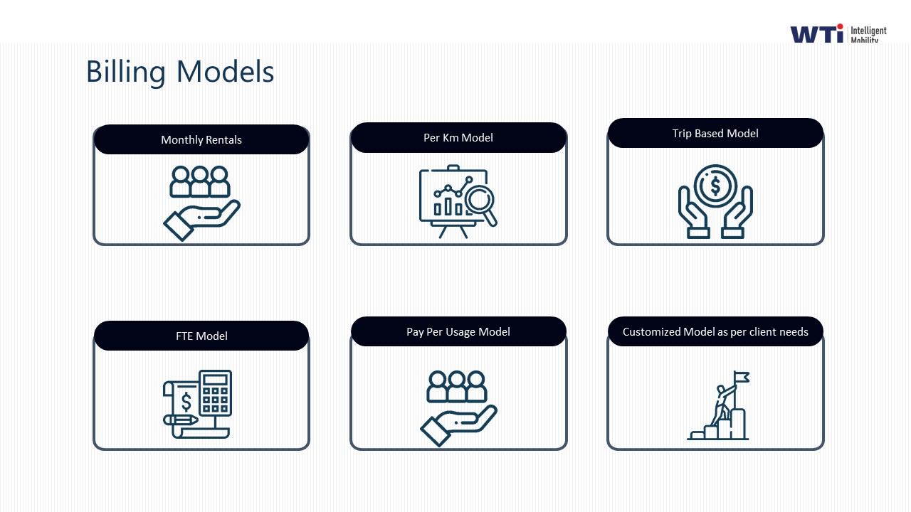
When leadership wants lower costs and higher reliability, how can ops explain real constraints like fleet buffers and Tier-2 supply without sounding defensive?
B0333 Explaining constraints to leadership — In India Employee Mobility Services (EMS), when leadership demands both lower CET/CPK and higher reliability, how should an operations leader explain the operational constraints (fleet buffers, time bands, Tier-2 supply limits) without sounding defensive or incompetent?
In Indian Employee Mobility Services, an operations leader should explain CET/CPK and reliability as two outputs of the same operating model, with explicit levers and constraints, rather than as conflicting emotions or excuses. The leader should translate buffers, time bands, and Tier‑2 supply limits into clear, quantified rules of thumb and trade‑offs that link directly to reliability, unit cost, and risk.
The most effective pattern is to frame operations as a governed system with defined levers. Fleet buffers, peak–off‑peak time bands, and vendor capacity in Tier‑2 cities should be positioned as design parameters that protect On‑Time Performance and safety. Reliability, fleet uptime, and Trip Adherence Rate depend on minimum buffer capacity, shift windowing, and vendor aggregation depth in each geography. If these parameters are driven below threshold, the system relies on last‑minute improvisation, which increases CET/CPK through dead mileage and emergency sourcing.
A common failure mode is explaining problems as one‑off incidents instead of recurring structural constraints. Most organizations see escalations when they under-specify peak window capacity, ignore hybrid-work volatility in rostering, or treat Tier‑2 and Tier‑3 supply as identical to metro supply. Leadership communication works better when the operations head shows how seat-fill, dead mileage, vendor tiers, and time-band SLAs interact to produce both cost and reliability outcomes.
A practical way to keep this non‑defensive is to present a small, stable set of operating rules and show the impact of flexing each rule. The discussion should focus on which constraints can be relaxed or re‑designed over time, such as vendor mix, EV/ICE fleet composition for high-mileage belts, or route-optimization intensity, rather than on assigning blame for individual failures.
- State target metrics upfront. Define desired OTP%, CET, and CPK baselines and confirm that these are the governing objectives for EMS.
- Map levers to outcomes. Show how fleet buffers, time-band capacity, vendor depth, and routing rules each affect OTP, dead mileage, and CET.
- Quantify constraints by band and city. Differentiate peak versus off‑peak and metro versus Tier‑2/3 in terms of realistic supply, SLA risk, and cost.
- Offer options with trade‑offs. Present 2–3 scenarios where higher buffers raise reliability and lower incident risk, while explaining the incremental CET/CPK change.
How do we quantify the cost of attendance instability from transport problems so Finance can weigh it against seat-fill/dead-mile savings?
B0334 Putting attendance instability in rupees — In India corporate employee transport (EMS), what’s the right way to quantify the financial exposure of attendance instability caused by transport issues—so Finance can compare it directly against the savings from aggressive seat-fill and dead-mile reduction targets?
In Indian corporate employee transport, the cleanest way to quantify financial exposure from transport-driven attendance instability is to translate every “late / absent due to commute” into three comparable unit metrics: cost per lost productive hour, cost per missed shift, and cost per escalation event. Finance can then compare these directly to savings from higher seat-fill and lower dead mileage, which are already measured in cost per km and cost per employee trip.
Most organizations start by defining a clear baseline using existing EMS and HRMS data. Transport logs identify trips delayed or missed due to routing, vehicle, or vendor failures. HRMS and attendance records map these events to late logins, partial shifts, or full-day absences. The result is a monthly count of “transport-attributed attendance incidents” and the total productive hours lost.
Finance teams then assign a monetary value to each lost hour using fully loaded cost per employee hour, not just salary. This includes wages, benefits, and any productivity-linked overheads that HR and Finance already track. For shift-based operations, where SLA penalties or lost revenue are relevant, an additional per-incident business impact factor is applied, such as missed output or client-facing SLA penalties.
Once this exposure is quantified, it can be put beside EMS optimization benefits that are already tracked, such as cost per km, dead-mile percentage, and seat-fill ratios. Aggressive seat-fill and dead-mile reduction lower the transport line item but can increase attendance volatility if they reduce buffers or routing resilience. A practical comparison uses three monthly curves: total EMS spend, loss from transport-driven attendance instability, and savings from optimization initiatives. This ensures cost-efficiency decisions do not ignore their impact on reliability, safety, and on-time performance, which remain primary EMS buyer priorities.
What usually causes dead miles to suddenly spike, and what simple controls can ops use to catch it early before Finance sees a budget overrun?
B0335 Preventing dead-mile spikes — In India EMS operations, what failure modes typically cause a sudden spike in dead miles (poor clustering, roster errors, vendor substitution gaps, last-minute cancellations), and how can operations build simple controls to stop the spike before Finance notices the overrun?
Dead-mile spikes in Indian EMS: common failure modes and simple operational controls
In Indian employee mobility services, dead miles usually spike when routing is forced to “react” to bad inputs such as broken rosters, fragmented vendor capacity, and last‑minute changes without guardrails. Operations can contain these spikes by putting simple, shift-level controls in routing, rosters, vendor allocation, and exception handling before costs ever reach Finance.
A frequent trigger is poor clustering of employees across shift windows. When transport teams route on outdated or manual lists, vehicles run half-empty or make long detours between far-apart clusters. Dead mileage also rises when hybrid-work attendance is not reflected in the routing engine in time, so cabs still move toward cancelled or no-show employees. Roster errors such as wrong addresses, duplicate entries, and mis-tagged shifts force re-routing on the fly, which adds empty kilometers between pickups.
Vendor substitution without clear geography or time-band rules is another failure mode. When the primary vendor is short on cabs, ad-hoc vendors may be dispatched from distant hubs, increasing garage-to-garage distance and off-route repositioning. Last-minute employee cancellations or late roster cut-offs amplify this, because the routing engine cannot re-pack seat capacity, so cabs travel with low Trip Fill Ratio between sparse pickups.
Operations can build simple controls by locking roster freeze times per shift and enforcing minimum seat-fill thresholds before route approval. A basic rule is to reject or re-cluster routes that breach set dead-mile caps or fall below defined Trip Fill Ratio. Centralized command centers can monitor a few live KPIs such as dead mileage share, Vehicle Utilization Index, and OTP%, and trigger micro re-routing only within pre-defined zone clusters, not across the city.
Vendor governance should assign each vendor to specific geographies and time bands with clear dead-mile baselines and substitution rules. EMS teams can further prevent spikes by integrating transport with HRMS so real-time attendance changes feed directly into roster optimization, reducing no-show runs. Short daily reviews on outlier routes with high dead miles help recalibrate shift windowing, fleet mix, and clustering before patterns become visible as cost overruns in Finance reports.
What controls help avoid monthly fights on trip distance and route adherence so CET/CPK billing becomes dispute-proof?
B0336 Dispute-proofing distance and route adherence — In India enterprise Employee Mobility Services (EMS), what are practical dispute-proof controls for trip distance and route adherence so CET/CPK doesn’t get stuck in monthly billing arguments between vendors, Finance, and site operations?
Dispute-proof control over trip distance and route adherence in Indian Employee Mobility Services comes from standardizing a single source of truth for trip data and tying billing to that source, not to manual entries or ad-hoc GPS screenshots.
Most organizations reduce CET/CPK disputes when every trip has a defined “trip ledger” that records planned vs actual route, distance, and time from the same telematics or app stack across all vendors. Billing then references that ledger ID and distance figure directly. This reduces room for argument between Finance, vendors, and site operations.
A common failure mode is allowing each vendor to use its own GPS or odometer figures. This creates mismatched records and forces manual reconciliations every month. Centralizing the data through a command center or mobility platform stabilizes distance measurement and route adherence checks. It also lets transport teams run random route adherence audits using the same dataset instead of debating vendor PDFs.
Disputes fall further when organizations set clear commercial rules upfront. Examples include defining chargeable distance from geo-fenced pick-up to drop, capping dead mileage, and treating approved route deviations in a consistent way. Finance teams gain control when CET/CPK is calculated from standardized trip categories and exception codes rather than free-form descriptions in invoices.
Practical controls that typically work are:
- Use a single routing and tracking source for all vendors. This can be a central EMS platform or command center feed that stores GPS traces, planned routes, and final trip distances for audit.
- Define a locked route map per shift and lane. Any deviation creates an exception flag that is visible in the same dashboard and must carry a documented reason code if it changes distance.
- Attach a unique trip ID and ledger entry to every duty slip. Vendors invoice only against these IDs, and Finance pays only for distances present in the ledger, not vendor-reported variants.
- Implement dead-mileage and detour policies. Examples are a maximum non-revenue distance per shift and pre-approved diversion bands before extra charges apply.
- Run automated route adherence and distance variance reports. Transport heads can use these for early alerts and to correct patterns before month-end billing.
These controls improve billing stability but introduce governance effort. Transport and Finance must align once on definitions, exception codes, and audit frequency. After that, most monthly billing arguments move from “whose numbers are right” to reviewing a shared dataset and closing only genuine anomalies.
How can leadership check if cost optimization is reducing workload for the transport team, not creating more monitoring and manual workarounds?
B0337 Testing if optimization reduces operational drag — In India corporate employee transport (EMS), how should an executive sponsor evaluate whether cost optimization initiatives are actually reducing ‘operational drag’ on transport teams, versus shifting effort into more monitoring, escalations, and manual workarounds?
An executive sponsor can distinguish real cost optimization from “operational drag” by tracking whether transport teams see fewer exceptions, faster closures, and less manual intervention across the ETS/EMS operation cycle, instead of more monitoring effort and workarounds. Genuine optimization improves OTP, dead mileage, and Trip Fill Ratio together with lower Cost per Employee Trip, while maintaining or reducing exception volume and escalation load.
Cost cuts typically create drag when they rely on manual controls, fragmented vendors, or weak routing tools. This usually shows up as more night-shift escalations, higher no-show and re-route rates, and frequent overrides to rigid routing or billing rules. When EMS is platformized properly, route optimization, rostering, and vendor governance are embedded in a governed operating model, so the 24x7 command center observes fewer red events and spends more time on trend analysis than firefighting.
A sponsor should insist on a before/after view of both economics and operations, with a small set of paired indicators that must improve together rather than in isolation.
Key signal pairs to review in QBRs and audits:
- Cost KPIs against reliability: CET/CPK vs OTP% and Trip Adherence Rate.
- Utilization vs effort: Vehicle Utilization Index and Trip Fill Ratio vs number of manual roster edits and ad-hoc dispatches per shift.
- Exception load: volume of SLA breaches, incident tickets, and vendor escalations vs total trips.
- Process automation: share of trips fully handled by the routing engine and apps vs trips processed by email/phone/manual sheets.
- People impact: overtime hours and night/weekend workload for the transport desk vs previous baseline.
If cost looks better but exception volume, manual touchpoints, and command-center workload rise, the sponsor is funding drag, not optimization.
What should IT and Finance ask for so CET/CPK, seat-fill, and dead-mile data stays consistent and month-end doesn’t turn into spreadsheets?
B0338 Keeping cost data consistent across systems — In India Employee Mobility Services (EMS), what should IT and Finance jointly ask for to ensure the data needed for CET/CPK, seat-fill, and dead-mile calculations is consistent across systems, so month-end reporting doesn’t become a spreadsheet reconciliation exercise?
IT and Finance teams in Indian Employee Mobility Services should jointly demand a single, governed trip-data model with API-level access, where every vendor and tool writes to the same canonical schema for trips, vehicles, and users. They should require that CET/CPK, seat-fill, and dead mileage are computed from this shared source of truth, not recreated separately in vendor portals, HRMS, and finance systems.
IT and Finance should first insist on a clearly documented canonical trip schema. The schema should standardize fields like trip ID, employee ID, vehicle ID, timestamps, distance, route, and cost attributes, and it should apply identically to EMS, CRD, ECS, and LTR data. This reduces data silos and stops each stakeholder from maintaining its own version of “what happened” for a given trip.
They should then require API-first integration into HRMS and ERP/finance systems. HRMS integration should align trips with rosters and attendance, and ERP integration should map trip and distance data directly into billing, GL codes, and cost centers. This keeps seat-fill and CET/CPK calculations consistent between operations dashboards and financial books.
Jointly, they should define a common KPI library and calculation logic. CET, CPK, Trip Fill Ratio, Vehicle Utilization Index, and dead mileage should have one agreed formula, owned by Finance and implemented by IT in the data pipeline. Vendors should not be allowed to redefine these metrics in their own reports.
Finally, IT and Finance should demand auditability and observability. The platform should store immutable trip logs, GPS traces, and calculation inputs, with role-based access and clear lineage from raw telemetry to reported KPI. This reduces month-end spreadsheet reconciliation and makes CET/CPK, seat-fill, and dead-mile numbers defensible in audits and board discussions.
If Finance wants tighter dead-mile caps but HR worries about longer rides and complaints, how do we agree on a compromise that protects attendance and avoids blame?
B0339 Negotiating dead-mile caps vs morale — In India enterprise EMS for shift-based commute, when Finance pushes for tighter dead-mile caps but HR worries about longer ride times and morale, how can stakeholders negotiate a compromise that protects attendance outcomes and avoids internal blame when complaints rise?
In India enterprise EMS, Finance and HR usually resolve dead-mile versus ride-time tension by agreeing on outcome-linked guardrails. The compromise works when dead-mile caps, maximum ride times, and attendance / EX metrics are fixed together and monitored from a single command view with clear SOPs for exceptions and escalations.
A common failure mode is treating dead-mile reduction as a pure cost lever. This often increases routing complexity, stretches ride times, and quietly erodes attendance, morale, and women-safety compliance. A better pattern is to set tiered dead-mile caps by shift window and route type, while hard-coding non-negotiables like maximum ride duration, night-shift women routing rules, and guard/escort logic into the routing engine and vendor SLAs.
Blame reduction depends on shared metrics and shared visibility. Most organizations create a small HR–Finance–Transport working group that signs off on a baseline “service envelope”. That envelope typically includes target OTP%, maximum ride time by band, dead mileage targets, safety incident thresholds, and a clear exception SOP when caps must be relaxed to hit shift adherence or safety obligations.
To keep this stable, stakeholders rely on centralized command-center operations and data-driven insights. Real-time NOC dashboards tracking OTP, trip-fill, dead mileage, exceptions, and complaints allow Transport Heads to rebalance trade-offs nightly. Outcome-based commercials indexed to OTP, safety, and seat-fill ensure vendors do not chase dead-mile savings at the expense of reliability or safety. HR can then defend the program with attendance and satisfaction evidence, and Finance can defend it with CPK and CET trends tied back to auditable trip and billing data.
After a weather disruption causes missed pickups, what questions should ops ask to separate unavoidable issues from preventable dead-mile or seat-fill planning mistakes?
B0340 Post-incident RCA for disruption variance — In India corporate employee transport operations (EMS), what post-incident questions should operations ask when a weather disruption causes missed pickups—specifically to separate unavoidable variance from preventable dead-mile and seat-fill planning errors?
In Indian corporate EMS operations, post-incident reviews after weather disruptions should isolate what no one could control from what routing and planning could have reduced. Operations teams should therefore ask distinct questions about demand, routing, capacity, and governance so that dead mileage, poor seat-fill, and vendor behavior are examined separately from genuine force‑majeure impact.
Operations should first reconstruct demand and exposure. They should ask how many shifts and employees were scheduled in the affected window, how many no-shows or cancellations occurred, and which routes consistently missed pickups. They should also ask when the first reliable weather or traffic alerts became available relative to roster freeze and dispatch cut-off times.
Routing and dead-mile analysis should focus on controllable planning choices. Operations should ask which routes saw the highest dead mileage, whether those routes could have been consolidated, and whether dynamic route recalibration was attempted once disruptions were known. They should also ask whether vehicles ran near-empty on long feeder legs, and whether hub-and-spoke deployment or temporary re-basing of vehicles could have reduced empty runs.
Seat-fill and capacity questions should separate pure disruption from structural over-supply. Teams should ask what average Trip Fill Ratio was on disrupted runs versus similar non-disrupted days, and whether extra buffer vehicles were deployed beyond agreed peak buffers. They should also ask whether hybrid-work attendance patterns were refreshed in the routing engine, or if static assumptions led to under-filled cabs.
Finally, governance and SOP questions should test if “assurance by design” failed. Operations should ask whether the command center escalated early enough, whether alternative shift-windowing or staggered reporting was requested from HR, and whether vendor partners adhered to contingency playbooks. They should also ask what exception data, GPS logs, and SLA reports show about response times, so that future EMS planning distinguishes inevitable weather variance from repeatable planning and execution gaps.
How can Finance set cost-model guardrails so CPK can’t be ‘improved’ by shifting dead miles to non-billable legs or changing pooled trip counting?
B0341 Guardrails against CPK manipulation — In India EMS programs, how can a finance controller set ‘guardrails’ in the cost model so a vendor cannot improve reported CPK by increasing dead miles on non-billable legs or by changing how pooled trips are counted?
In Indian Employee Mobility Services, a finance controller prevents artificial CPK improvement by hard-coding how distance, trips, and pooling are defined and audited, and by tying payouts to verified telematics data and utilization KPIs instead of vendor-reported summaries. The cost model must separate chargeable vs non-chargeable distance, define a canonical “trip unit,” and link payments to KPIs like dead mileage, Trip Fill Ratio, and route adherence that are computed from raw GPS and trip logs rather than invoices alone.
A common failure mode is letting vendors bill on loosely defined “per km” or “per trip” slabs without explicit rules for dead mileage and pooling. Vendors can then park vehicles far from hubs, increase non-billable legs to optimize their own operations, or split and merge pooled trips on paper to lower apparent CPK while increasing total kilometers and cost per employee trip. Finance loses control when definitions differ between vendor MIS, transport operations, and Finance systems, and when there is no unified data model for trips, kilometers, and seats.
Guardrails work best when defined as contractual rules plus calculable metrics. The contract can specify a dead-mile cap per shift window, a single definition of an EMS trip, minimum seat-fill thresholds, and an obligation to expose raw GPS and trip data via API. Payments can then be indexed to verified CPK, CET, Trip Fill Ratio, and dead-mileage ratios, with penalties for breaching caps or for under-reporting pooled capacity. This shifts optimization behavior towards reducing genuine cost per employee trip instead of reshaping distance accounting.
Key guardrails a finance controller can embed include:
Canonical distance rules.
Define exactly which legs are billable and which are not. Mandate that start and end odometer or GPS points are the employee pickup and drop boundaries, not the vendor’s garage. Cap allowed non-billable repositioning distance per route or per shift window, and treat excess as billable or as a penalty driver.
Standardized trip and pooling definitions.
Define an EMS trip as a single rostered route run within a shift window with a specified list of employees and stops. State that a pooled trip is one physical vehicle run with N manifested employees, not N separate “virtual trips,” and that CPK and CET will be calculated at vehicle-run and seat level, not at abstract booking level.
Utilization and dead-mile KPIs.
Make Vehicle Utilization Index, Trip Fill Ratio, and dead mileage ratio explicit KPIs in the commercial model. Link a portion of payouts or incentives to hitting agreed thresholds on these KPIs, which are computed from GPS and roster data. This deters vendors from trading higher dead miles for a lower apparent CPK.
Unified data and audit requirements.
Require trip-level data feeds from the routing platform or command center, including manifest, GPS trace, and timestamps. Specify that Finance will calculate CPK and CET from this canonical dataset, and that vendor invoices must reconcile to this ledger through clearly mapped IDs. Reserve the right to run route adherence audits and random route audits against raw telematics logs.
Outcome-linked payment logic.
Structure the commercial model so that base CPK is only one component. Introduce bonuses or penalties linked to on-time performance, seat-fill, and dead-mile caps instead of pure distance. This reduces the incentive to game distance accounting and aligns vendor economics with real cost per employee trip.
What signs tell us better seat-fill is starting to hurt attendance (longer rides, late logins, no-shows), and how can HR track this without it becoming a surveillance argument?
B0342 Spotting when seat-fill hurts attendance — In India corporate employee commute (EMS), what practical indicators show that improved seat-fill ratios are starting to harm attendance—such as increased average ride time, higher late logins, or rising no-shows—and how should HR operationalize those indicators without turning it into a surveillance fight?
Most organizations know seat-fill has gone too far when reliability and basic “commute comfort” start degrading at the same time as KPIs look artificially good. A practical rule is that if pushing higher seat-fill coincides with longer average ride times, more late logins, and rising no-shows or cancellations on specific routes or shifts, then optimization is starting to hurt attendance rather than help it.
The earliest indicators usually show up in operational and HR-linked data, not in one big incident.
Concrete operational signals include:
- Average ride time creeping up beyond agreed caps for key corridors or timebands, especially for women on night shifts.
- On-Time Performance (OTP) falling for the first/last few pickups on highly pooled routes, even though “overall” OTP looks acceptable.
- Dead mileage reducing sharply while exception tickets, reroutes, and manual interventions from the transport desk increase.
- High Trip Fill Ratios on paper, but more mid-route changes, re-sequencing, or extended detours reported by drivers and the command center.
Attendance and HR-facing signals include:
- Late logins clustering around particular routes, zones, or shift windows after routing changes or new pooling rules.
- No-show and cancellation rates rising on routes with the highest seat-fill, while other routes remain stable.
- More commute-related complaints in floor connects, transport helpdesk logs, or HR grievance channels that mention “long routes,” “too many pickups,” or “unreliable timings.”
- Attendance volatility or short-notice WFH requests increasing in teams that rely heavily on specific high-pooled routes.
To operationalize these indicators without creating a surveillance battle, most HR and Transport teams treat them as service-quality thresholds, not employee-behavior monitors. The practical approach is to define a small set of shared guardrails that link routing decisions to HR outcomes while keeping individual-level data usage minimal and transparent.
Typical guardrails include maximum ride-time targets by distance band and shift type, minimum OTP thresholds for first and last pickups, and an agreed ceiling on Trip Fill Ratio for sensitive night-shift or women-heavy routes. HR, Transport, and the vendor then review these metrics at a corridor or cluster level rather than by named employee, using dashboards and command-center reports to flag when a particular route or shift consistently breaches thresholds.
In practice, this works best when HR’s role is framed as setting “employee safety and comfort standards” and validating patterns, while Transport and the vendor adjust the routing engine, fleet mix, and pooling rules. HR can push for structured reviews when three or more indicators degrade together on the same route group over a defined period, such as rising average ride time, declining OTP, and increased late logins for the same shift window.
To avoid a surveillance narrative, organizations generally take three additional steps. First, they publish clear commute principles—such as maximum acceptable ride times, night-shift safety rules, and how data is used—so employees understand the boundaries. Second, they anchor decisions in anonymized or aggregated patterns, using feedback tools, floor connects, and user satisfaction indices to validate numbers. Third, they ensure that any individual-level data pulled (for example, repeated no-shows) is handled through existing HR and manager channels, not through new, opaque monitoring practices.
When these indicators are embedded in regular governance—QBRs with vendors, joint HR–Transport reviews, and command-center dashboards—they become early-warning tools. This allows teams to step back seat-fill, adjust routes, or add buffer capacity on critical corridors before commute dissatisfaction starts to damage attendance, safety perception, or employer brand.
For our EMS program, how can Finance connect CET/CPK savings to real changes in attendance and productivity, not just separate reports?
B0343 Link cost to productivity — In India’s corporate Employee Mobility Services (EMS), how do Finance teams credibly link cost per employee trip (CET) and cost per kilometer (CPK) improvements to measurable attendance stability and productivity outcomes, instead of treating them as separate dashboards?
In Indian corporate Employee Mobility Services, Finance teams link cost per employee trip and cost per km to attendance and productivity only when commute data, HRMS data, and SLA metrics are modeled in a single, reconciled view of each trip and shift. Finance stops treating CET/CPK as isolated dashboards when every rupee of transport spend is mapped to specific employees, shifts, and on-time performance outcomes with traceable evidence.
Finance teams that succeed usually start by insisting on a common trip ledger. This trip ledger joins vendor bills, GPS trip logs, and command-center SLA data with HRMS shift rosters and attendance records for each employee. Once that linkage exists, Finance can calculate cost per attended shift, cost per productive hour, and incremental cost of late arrivals or no-shows, instead of watching CET and CPK in isolation.
The most credible narratives use a small set of stable, Finance-owned indicators. A frequent pattern is to track three linked time-series: CET/CPK, on-time performance and exception closure, and shift adherence or late-login rates from HRMS. When CET reduction coincides with flat or better OTP and equal or lower late-login rates, Finance can present savings as productivity-neutral or productivity-accretive. When aggressive CET cuts show a rise in missed pickups, extended trip times, or late logins, Finance can quantify “false savings” by estimating lost productive minutes per employee and converting that into monetary impact per site or process.
A common failure mode is treating HR, Transport, and vendor dashboards as independent truths. In practice, Finance needs a single reconciled KPI layer where trip, SLA, safety, and attendance fields are locked to one reference ID per trip. That layer allows Finance to create site-wise or process-wise views that compare business units with similar work profiles but different CET/CPK and OTP, revealing where lower unit costs genuinely support stable attendance and where they damage it. Over time, this enables outcome-based contracts where a portion of vendor payouts is indexed not only to CPK and CET, but also to jointly agreed on-time and exception-closure thresholds that protect attendance stability as a core business outcome.
When seat-fill looks fine but CET/CPK still goes up, what usually causes it and how do we quickly diagnose it without spreadsheet firefighting?
B0344 Seat-fill vs cost mismatch — In India’s corporate ground transportation programs, what are the most common reasons seat-fill ratio targets look good on paper but CET/CPK still rises in practice, and how should Operations and Finance diagnose that mismatch without months of manual reconciliation?
In Indian corporate mobility programs, seat-fill ratios often look healthy while cost per employee trip (CET) and cost per km (CPK) rise because utilization metrics are calculated on a narrowed slice of trips, while dead mileage, exceptions, and fragmented demand sit outside that calculation and still hit the P&L. Operations and Finance can diagnose this mismatch by standardizing a small set of shared KPIs, reconciling them via trip-level telemetry and billing data, and using command-center style dashboards instead of manual spreadsheets.
The most common pattern is that seat-fill is measured only on “rostered” or “planned” trips. Dead mileage from repositioning, under-utilized late-night returns, no-shows, and ad-hoc CRD or ECS movements are excluded. This inflates the apparent Trip Fill Ratio while CET and CPK reflect the full journey and duty cycle. Another failure mode is misaligned service catalogs, where EMS routes are optimized but parallel LTR or CRD usage for the same corridors runs at low utilization, pushing aggregate unit costs up despite good seat-fill on the main program.
Data fragmentation across EMS platforms, CRD providers, and project/event shuttles is a consistent root cause. HRMS data, GPS logs, and vendor invoices are not reconciled under one semantic layer, so Finance sees cost inflation but cannot tie it back to route design, shift windowing, or vendor behavior. Command-center operations and data-driven insights exist in many programs, but without a shared, reconcilable definition of “trip,” “seat,” and “km,” seat-fill becomes an isolated metric rather than a cost-governance tool.
A practical diagnostic approach for Ops and Finance is to agree on a short, joint KPI set and a minimum data model before going into detail. They can start by aligning on definitions for Trip Fill Ratio, Vehicle Utilization Index, dead mileage, and Cost per Employee Trip across EMS, CRD, ECS, and LTR. Then they can pull a 4–8 week sample of trip-level and billing data through a single dashboard or data extract, where each trip includes planned vs actual distance, passenger count, dead-km tags, and cost allocation.
Operations can then segment CET and CPK by route type, shift window, and vendor, and overlay no-show rates, exception trips, and off-roster movements. Finance can validate that billed km and trips tie back to GPS and roster data, not just vendor summaries. This approach turns the command center from a real-time control room into a retrospective cost and compliance audit layer, without requiring a one-time, months-long manual reconciliation.
To keep the exercise contained and repeatable, many teams use a simple, recurring review loop rather than a one-off cleanup. They run a monthly “mobility cost and utilization” huddle where the Transport Head, Finance Controller, and Procurement review seat-fill, CET, CPK, dead mileage, and SLA breach rate on the same dashboard. Exceptions that consistently show high cost with normal seat-fill are tagged for route redesign, vendor rationalization, or contract model changes, such as shifting specific corridors from EMS to LTR or from per-trip to per-seat models.
Over time, this joint diagnostic loop shifts seat-fill from being a vanity metric to a leading indicator tied to real unit economics. CET and CPK stop drifting because every variance is traceable to operational levers like routing, fleet mix, hybrid-work demand patterns, and vendor behavior, all visible through a shared data and governance model rather than ad-hoc spreadsheets.
images:
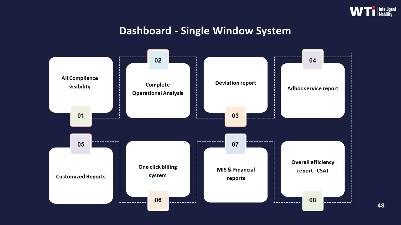
How should our CFO validate dead-mile savings claims and make sure they show up in billing, even with weekly hybrid roster changes?
B0345 Validate dead-mile savings — For India-based EMS route-to-office transport, how can a CFO pressure-test vendor claims of dead-mile reduction to ensure the savings are real, repeatable, and auditable at invoice time—especially when hybrid rosters change weekly?
For India-based employee mobility, a CFO can pressure-test dead-mile reduction claims by demanding route-level data, baselines, and audit trails that reconcile directly to invoices, not just high-level PPT metrics. The tests must link vendor routing outputs, telematics traces, and billing logic so that every “saved kilometre” is independently verifiable despite weekly hybrid-roster changes.
First, the CFO should insist on a clear baseline before any optimization. The baseline should quantify historic dead mileage, cost per kilometer, and cost per employee trip under current EMS operations. The baseline must be locked with written assumptions such as shift windows, seat-fill norms, fleet mix, and attendance variability. Dead-mile reduction claims are unreliable when vendors skip a measurable “before” state.
Second, any vendor promising reduced dead mileage should expose how routing decisions are made. The CFO should ask for documentation of the routing engine’s logic, including shift windowing, seat-fill targets, and caps on dead mileage per cab. The vendor should show how dynamic route recalibration works when rosters change day to day. A common failure mode is when algorithms look efficient on static rosters but break under hybrid attendance volatility.
Third, the CFO should require a canonical data structure for trips that makes dead mileage auditable. Each trip should have start and end coordinates, tagged distance for live legs versus empty legs, and timestamps aligned with the EMS operation cycle. Trip adherence rate and on-time performance should be measurable from the same dataset. Dead-mile reduction can only be trusted when it uses the same underlying telemetry that drives SLA reports and not a parallel, vendor-controlled metric.
Fourth, invoice-time verification must become non-negotiable. The CFO should ask for billing models that explicitly separate chargeable live kilometers from non-chargeable dead kilometers where the vendor is claiming reductions. The billing system should support tariff mapping and online reconciliation tied to the trip ledger. A frequent risk is opaque billing where “optimized” operations still bill the enterprise as if nothing changed.
Fifth, the CFO should design outcome-linked commercials around dead-mile metrics. Contracts can index a portion of payouts to quantitative indicators such as cost per employee trip, vehicle utilization index, and trip fill ratio. A vendor who is confident in dead-mile reduction should accept incentives and penalties that move with these metrics over a defined review window. This structure discourages tokenistic claims and focuses on measurable, repeatable outcomes.
Finally, the CFO should align Finance, Transport, and IT on a shared verification model. Transport and EMS operations should validate that routes remain operationally realistic. IT should confirm that data pipelines from routing, telematics, and billing are traceable and tamper-evident. Finance should test that monthly dead-mile and cost-reduction figures can be reproduced independently from the raw trip logs during audit. Vendors that cannot support this level of observability typically fail when hybrid rosters become more volatile.
images:
What are the usual leakage points that push up CET/CPK—like no-shows or ad-hoc trips—and what controls actually stop them in day-to-day operations?
B0346 Leakage sources and controls — In India’s corporate employee commute operations, what leakage sources typically drive CET/CPK inflation (for example: no-shows, last-minute ad-hoc trips, route deviations, duplicate manifests), and what practical controls do mature programs use to prevent those leakages?
In Indian corporate employee commute operations, cost per employee trip (CET) and cost per kilometer (CPK) inflate when unobserved operational leakages accumulate across the trip lifecycle. Mature programs treat each leakage as a controllable failure mode and combine process SOPs with platform controls, auditability, and command-center oversight to contain them.
The most common leakage sources sit around routing, utilization, and exceptions. Under-filled cabs, dead mileage between trips, and static routing in hybrid-work environments push CPK up even when vendor rates look competitive. Late roster changes, no-shows, and last-minute ad-hoc trips trigger unplanned vehicles or extended detours, which silently raise CET and create billing disputes. Route deviations, fragmented vendor ecosystems, and manual duty slips create opportunities for inflated kilometers, duplicate manifests, and misaligned invoices, especially where GPS or app data is not the single source of truth.
Mature EMS/ETS programs respond with a few practical guardrails. Dynamic route optimization and seat-fill targets limit dead mileage and underutilization, especially when rosters are integrated with HRMS and shift systems. Central command centers monitor on-time performance, route adherence, and exception alerts in real time, and they enforce escalation matrices that cap how much deviation or extra running can be approved on the fly. Centralized billing with tariff mapping, automated tax calculations, and SLA-linked reconciliation reduces scope for duplicate or mismatched entries and makes CET/CPK variance traceable to specific trips and vendors.
Controls that work in practice tend to be simple but enforced consistently. Typical measures include mandatory app-based trip start/stop with GPS logs, OTP-based trip verification, and automated geofence or tamper alerts to reduce manual overrides. Maker–checker processes on fleet induction and compliance reduce unplanned breakdowns that often lead to costlier backup trips. Outcome-linked commercials that tie payouts to seat-fill, dead mileage caps, and on-time performance shift some leakage risk back to vendors while preserving transparency through auditable trip ledgers and dashboards. Over time, these mechanisms make CET and CPK the output of governed operations and data-driven routing, rather than a moving target driven by daily firefighting.
images:
How do we plan for festivals and monsoon so our CET/CPK targets don’t break when attendance and travel times suddenly change?
B0347 Festival and monsoon sensitivity — In India’s EMS shift-based routing, how should Facilities/Transport Heads run sensitivity analysis for festival seasons and monsoon disruptions so that CET/CPK targets don’t collapse when attendance patterns and travel times spike?
In India’s EMS shift-based routing, Facilities and Transport Heads should run sensitivity analysis by stress-testing key routing and cost variables against worst-case festival and monsoon scenarios before the season starts. The core principle is to pre-model “what if” spikes in attendance, no-shows, and travel time against CET and CPK thresholds, and then lock season-specific routing, fleet, and commercial guardrails into SOPs.
Sensitivity analysis works when it is built on the same KPIs used in everyday EMS governance. Transport teams should model how On-Time Performance, Trip Adherence Rate, Trip Fill Ratio, dead mileage, and Vehicle Utilization Index change under longer travel times, flooded routes, and temporary road closures. Command-center data, dynamic route recalibration patterns, and past deviation and service reports provide the baseline for these simulations.
The main trade-off is between reliability and unit cost. Higher peak buffers and standby fleets protect OTP and safety but can dilute vehicle utilization and increase cost per employee trip. Facilities Heads should, therefore, define explicit trigger bands, such as “if average ETA on core corridors rises by 20%, allow extra buffer vehicles but cap dead mileage at a defined level.” Commercial models should incorporate season-specific clauses for peak operations so that outcome-based contracts still index payouts to service reliability, safety incidents, and seat-fill, even when shift windowing and routing change.
A practical festival and monsoon SOP for sensitivity analysis usually includes:
- Pre-season baselining of CET, CPK, OTP, and dead mileage by corridor and shift window.
- Scenario modeling of 10–30% attendance shifts and 15–40% travel-time inflation on critical routes.
- Command-center playbooks for dynamic rerouting and capacity reallocation under live weather and traffic alerts.
- Temporary fleet-mix rules that prioritize higher-capacity vehicles on high-risk, high-delay corridors.
- Daily review loops where deviations from modeled scenarios trigger rapid routing and roster adjustments.
images:
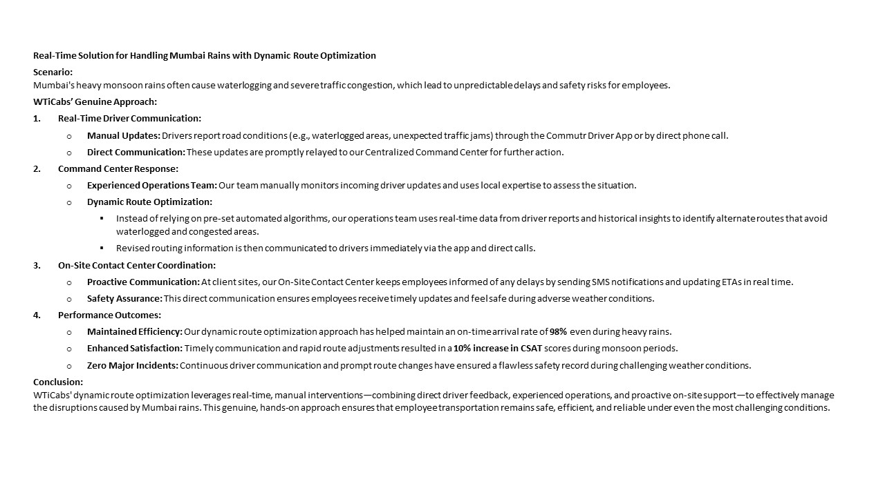
In Tier-2 locations, what constraints usually blow up the cost model, and how can Procurement check if the vendor’s CET/CPK assumptions are realistic?
B0348 Tier-2 cost model realism — For India’s corporate EMS programs serving Tier-2 cities, what Tier-2 routing constraints (permit boundaries, sparse supply, longer dead miles, limited night availability) most often break cost models, and how should Procurement evaluate whether a vendor’s CET/CPK assumptions are realistic?
For corporate EMS in India’s Tier-2 cities, the routing constraints that most often break cost models are long dead mileage between clusters, permit and boundary restrictions that block “ideal” routes, sparse and time-limited vehicle supply, and fragile night-shift availability that collapses under real attendance patterns. These constraints inflate cost per km (CPK) and cost per employee trip (CET) when they are not explicitly modelled in vendor assumptions and commercials.
In Tier-2 EMS, dead mileage usually spikes because employee homes are scattered and fleet hubs are few. This increases unbilled kilometres before first pick-up and after last drop. Permit limits and municipal boundaries can force detours or specific entry/exit points, which break clean, circular routes. Sparse supply means vehicles are repositioned across town to cover shift windows, and this repositioning is often omitted from vendor CET. Limited night availability combines with driver fatigue rules and women’s safety norms to create additional constraints like escorts and specific routing rules.
Procurement teams should test CET/CPK realism by asking vendors to present city-specific routing simulations and historic OTP/seat-fill data for comparable Tier-2 locations. Procurement should require explicit dead-mileage assumptions, average trip fill ratios, and buffer capacity policies for night shifts. Any vendor proposal that assumes metro-like pooling efficiency, ignores permit-driven detours, or shows unusually low dead mileage in a spread-out Tier-2 map is likely to understate true costs. Evaluations should favour vendors who can show integrated command-center operations, real-time routing control, and data-backed performance in similar Tier-2 EMS programs.
How do we set a clean CET/CPK baseline before we change pooling or routing, so Finance can prove what savings came from the program vs. attendance changes?
B0349 Define CET/CPK baseline — In India’s employee mobility services, how do you set a defensible baseline for CET/CPK before changing routing rules or pooling logic, so Finance can attribute savings to the program rather than to headcount or hybrid attendance swings?
In India’s employee mobility services, a defensible CET/CPK baseline is built by fixing a time-bounded “pre-change” window, normalizing all trips for attendance and shift mix, and locking that dataset as the reference cohort before any routing, pooling, or fleet-mix interventions go live. Finance can then attribute savings to the program only when post-change unit economics improve against the same normalized demand profile.
A robust baseline starts with explicit scope. Organizations define which sites, shifts, and employee categories are in-bounds, then choose a representative period, usually 8–12 weeks, with “steady state” rosters and no major policy changes. All EMS trips in this window are captured with raw fields such as passengers per trip, kilometers, route type, shift band, and vehicle category, because CET and CPK depend heavily on these operational drivers.
Normalization is where most baselines fail. Attendance, hybrid-WFO patterns, seasonality, and temporary hiring surges are separated as demand variables. Finance and transport teams then segment the data into stable cohorts, for example “night shifts – DC 1 – 6-seater MUV,” and compute CET and CPK within each cohort. This creates a matrix of cell-level baselines that already factor in typical seat-fill, dead mileage, and OTP/SLA expectations.
Once this matrix is agreed and signed off by Finance as the “baseline book,” routing rules, pooling logic, or EV/ICE mix can be changed. Post-change performance is compared cell-to-cell, not at a crude monthly total. If total cost drops only because headcount reduced or WFH increased, cohort CET/CPK will look unchanged. If routing and pooling improved, CET/CPK will fall even after re-weighting the cohorts by current attendance, which gives Finance a defensible attribution to the program rather than to volume swings.
images:
What early signals should Ops watch so we can spot a CET/CPK blowout coming—like seat-fill drift or dead-mile creep—before it becomes a night escalation and billing mess?
B0350 Early warning cost signals — In India’s corporate EMS, what leading indicators should a Transport Operations team monitor to predict a coming CET/CPK blowout (for example, seat-fill drift, roster volatility, dead-mile creep) early enough to avoid 3 a.m. escalations and end-of-month billing shocks?
In India’s corporate Employee Mobility Services, transport operations teams avoid CET/CPK blowouts by watching a small set of leading indicators that move before the invoice does. The most predictive indicators sit around utilization, routing quality, roster stability, and policy drift, and they should be visible in the command center on a shift-by-shift basis, not only in MIS at month-end.
The strongest early warnings usually emerge from utilization and routing. Seat-fill percentage per route and per timeband is a primary indicator. A consistent drop in Trip Fill Ratio signals rising cost per employee trip long before bills spike. Dead mileage as a share of total kilometers is another leading signal. An upward trend in empty runs between hubs, last pick-ups, and first drops indicates route inefficiency and poor hub-and-spoke design. When routing engines start missing original dead-mile caps or route adherence audits show more detours and re-routing, it usually precedes higher CPK.
Roster and demand volatility create the second cluster of signals. Frequent late roster changes, high no-show rate, and rising ad-hoc or emergency trips point to a growing gap between planned capacity and actual demand. Hybrid-work patterns that cause shift windowing to spread out can reduce pooling density and push per-seat economics into red. Daily exceptions logged by the command center for off-roster pickups or manual overrides in the routing engine are strong precursors to CET drift.
A third set of indicators sits in vendor, fleet, and driver behavior. Decreasing Vehicle Utilization Index, more standby cabs being activated to save OTP, and higher driver attrition or fatigue index all push the system towards inefficient, short-notice deployments. Early patterns in fleet uptime drops or maintenance cost ratio increases often cause last-minute vehicle swaps, which expand dead mileage and reduce pooling opportunities. Vendor SLA breach rate on response time or fleet availability is another quantitative predictor of cost escalation.
Safety and compliance indicators also have cost consequences. Rising incident rate, more escort-requirement overrides, and tighter night-shift routing constraints can compress pooling and force additional vehicles into sensitive routes. When security or EHS teams adjust geo-fencing and escort rules without corresponding route-policy recalibration, it can quietly add new constraints that the routing engine solves with more cabs rather than better clustering, inflating CET.
To turn these signals into practical early alerts, most organizations need a simple, shift-based dashboard in the command center. The dashboard should show, for each timeband and major hub, live seat-fill, dead mileage, vehicle utilization, no-show rate, OTP vs buffer usage, and number of ad-hoc trips triggered. Thresholds and trend lines matter more than single values. A one-week upward trend in dead-mile percentage or a three-shift drop in seat-fill is a more reliable predictor than a single bad day. Centralized NOC teams should run short daily huddles to review these trends, flag routes crossing thresholds, and push rapid experiments in routing, fleet mix, or roster rules before patterns become embedded.
Commercial models and procurement design influence which indicators matter most. Where contracts are per-kilometer, dead-mile creep and low utilization are primary risks. Where contracts are per-seat or per-trip, no-show rates, seat-fill drift, and hybrid attendance volatility dominate. In outcome-linked contracts, SLA breach penalties, incident-linked penalties, and OTP buffers can create hidden cost through over-servicing. Transport heads who maintain a simple mapping from each commercial lever to 3–5 associated operational indicators maintain better control and can discuss cost risks with Finance using shared language.
Across all of this, the main failure mode is treating these metrics as monthly MIS rather than live controls. When seat-fill and dead mileage are only visible in post-facto reports, Transport teams are forced into reactive explanations instead of preventive action. When the same metrics are made visible in real time to the command center, with clear SOPs on what to do when thresholds are crossed, teams gain the “operational calm” needed to avoid 3 a.m. escalations and end-of-month billing shocks.
images:
HR wants shorter rides and fewer stops, but Facilities wants more pooling to cut CET—how do we resolve that conflict without it turning into a blame game when employees complain?
B0351 HR vs Facilities pooling trade-off — For India’s corporate commute programs, how do HR and Facilities resolve the conflict where HR wants better employee experience (shorter ride times, fewer stops) but Facilities is pushing pooling to improve seat-fill and CET—without turning it into a political fight after complaints?
For Indian corporate commute programs, HR and Facilities resolve the “experience vs pooling” conflict fastest when they move from opinion-based arguments to a single, shared KPI framework with explicit thresholds for both employee experience and cost. The conflict reduces when seat-fill and Cost per Employee Trip (CET) targets are set alongside hard guardrails on On-Time Performance (OTP), maximum ride time, and safety compliance, and when both teams review these metrics together in a fixed governance cadence.
A common failure mode is debating “too many stops” or “employees are unhappy” without data that links routing choices, seat-fill, and complaints. Another failure mode is optimizing purely for pooling and CET, which often increases dead mileage and incident risk, and eventually creates HR escalations and reputational noise. Governance usually stabilizes when HR, Facilities, and Finance agree on a basic service catalog for EMS with clearly differentiated pooling levels, entitlements by persona, and shift windows, instead of a one-size-fits-all pooling policy.
A practical pattern is to run routing and pooling through a central command-center playbook, where Transport owns day-to-day seat-fill and dynamic routing, HR owns safety and Commute Experience Index (CEI), and Finance owns CET and cost-per-kilometre, but all three see the same trip-level dashboards. It also helps to implement pilot routes where higher pooling is allowed only if OTP, maximum ride duration, and complaint closure SLAs remain within agreed thresholds over a defined review period. When complaint patterns or CEI scores cross pre-set triggers, the SOP should mandate automatic de-pooling or route redesign, rather than ad-hoc blame.
What’s a practical low-toil way to handle exceptions like no-shows or shift swaps, while still keeping a clean audit trail from the exception to the route change to the invoice?
B0352 Low-toil exception handling — In India’s EMS operations, what is a practical ‘two-click’ process design for exception handling (no-show, address change, shift swap) that reduces manual toil while still keeping audit-ready linkage between the exception, the route change, and the final invoice?
In India’s EMS operations, a practical “two-click” exception process design routes every no-show, address change, or shift swap through a single exception form and a single approval action. The exception record drives automatic route recalculation and billing changes, and the platform then locks all three together in an immutable trip ledger for audits.
A robust pattern starts with a dedicated exception button inside the transport command center or admin app. The first click opens a structured exception form that is pre-populated with trip ID, employee ID, current roster, and planned route. The operator only selects an exception type such as no-show, address change, or shift swap and fills a minimal required field like new address or replacement employee code.
The second click is a confirm or approve action that writes an exception record into the trip ledger and triggers an automated workflow. The routing engine recalculates the active route based on the updated pickup list and sequence. The EMS platform also recalculates billable distance, dead mileage, and cost per employee trip according to configured commercial rules.
The system should then generate an audit-ready chain that links four elements using one unique trip-exception ID. The first element is the original roster and route. The second element is the exception record with timestamp, user ID, and reason code. The third element is the recalculated route and updated telematics trace. The fourth element is the final invoice line item and tariff logic applied. This linkage enables Procurement, Finance, and Audit teams to reconstruct why a deviation occurred and how it affected cost.
To keep daily toil low for Facility and Transport Heads, the exception form can expose only standardized reason codes and mandatory fields. Supervisors can monitor exception volumes and closure SLAs on a command-center dashboard, while HR and Finance receive summarized exception reports that are directly reconciled with billing and on-time performance metrics.
How can Finance catch silent dead-mile leakage like empty repositioning or detours, without making Ops feel policed and defensive?
B0353 Controls without ops backlash — For India’s corporate ground transportation billing, how should Finance structure controls to catch ‘silent’ dead-mileage leakage (empty repositioning, unapproved detours, extended waiting) without creating an adversarial relationship with the Transport Operations team?
Finance should treat dead-mileage control as a shared “physics of the operation” problem with Transport, not a fraud hunt, and anchor controls in transparent data definitions, pre-agreed rules, and exception-based reviews. Finance teams that succeed create a single, auditable view of distance and time, then link commercials to that view with clear caps and playbooks, instead of line‑item policing after the fact.
Finance can start by insisting on a canonical trip ledger that merges GPS/telematics data with booking and roster metadata. This ledger should expose booked distance, actual distance, dwell time, and route adherence for each trip, which allows dead mileage, detours, and waiting to be quantified as specific fields rather than inferred in Excel. Central command‑center tooling, trip adherence rate, and route adherence audits can supply much of this data.
Controls work best when the commercial model is explicit about what is payable. Finance and Transport can codify rules such as permissible garage‑to‑garage buffers, maximum detour percentages, and free versus billable waiting slabs by service type, shift band, or city. Once this is agreed as policy, Finance can configure billing engines and reconciliation reports so that only deviations beyond those thresholds surface as exceptions.
To avoid an adversarial tone, Finance should review patterns, not individuals. Periodic joint reviews with Transport that look at cost per kilometer, cost per employee trip, dead‑mileage ratios, and SLA breach rate help distinguish structural routing issues from genuine leakages. When the same dashboards also track on‑time performance and fleet uptime, Transport sees that the goal is to rebalance cost, reliability, and safety, rather than to second‑guess every operational decision.
What proof should Procurement ask for that seat-fill optimization won’t hurt attendance or late logins, and how can we put that into SLAs without making the contract unmanageable?
B0354 Seat-fill SLAs vs attendance — In India’s EMS vendor governance, what should Procurement require as evidence that seat-fill optimization won’t degrade attendance or productivity (for example, increased ride time causing late logins), and how do you write that into SLA language without overcomplicating the contract?
Procurement should require data-backed proof that seat-fill optimization preserves shift adherence and does not extend ride times to the point where attendance or productivity is hit. Procurement should then encode a few simple, outcome-linked SLAs that cap ride-time and protect login punctuality, instead of trying to regulate the optimization algorithm itself.
The most practical evidence set focuses on three areas. First, historical OTP% and Trip Adherence Rate for similar EMS programs should be provided, with and without pooling or optimization. Second, vendors should submit anonymized samples of route plans showing seat-fill levels against ride-duration bands, along with shift start times. Third, vendors should provide complaint and escalation statistics linked to “long ride” or “late login” reasons, along with current corrective SOPs.
Contractually, the SLAs should bind the vendor to outputs that matter to HR and Transport, not to how the routing engine works. A concise structure is to define maximum ride-time bands by distance or zone, a minimum OTP% tied to shift start, and an exception-closure SLA for late-login incidents attributable to transport. These should sit alongside standard reliability and safety clauses to keep the document readable.
Procurement can keep language tight by focusing on 3–5 measurable KPIs and simple remedies. For example, a single annexure can define how OTP%, ride-duration, and exception counts are calculated, how many periods of non-compliance trigger penalties, and how data will be shared with HRMS or attendance systems. This avoids algorithm detail while still giving Finance, HR, and Transport clear levers for vendor governance.
From an IT angle, how do we check if the data behind CET/CPK and seat-fill is reliable—GPS, trip logs, roster source-of-truth—so we don’t optimize on bad data?
B0355 Trustworthiness of cost data — For India’s corporate EMS programs, how should a CIO evaluate whether the data feeding CET/CPK and seat-fill metrics is trustworthy (GPS integrity, trip logs, roster source-of-truth), so the business doesn’t make routing decisions on dirty data?
For corporate EMS in India, a CIO should treat CET/CPK and seat‑fill metrics as untrusted by default until the GPS stream, trip logs, and roster sources are proven consistent, tamper‑resistant, and reconcilable end to end. Trustworthy data exists only when every trip can be traced from roster creation to GPS trail to billing record without unexplained gaps or manual edits.
A common failure mode is when roster data, GPS tracks, and billing systems operate as silos. This often causes dead mileage to disappear, no‑shows to be misclassified, and seat‑fill to be overstated. Another frequent weakness is ungoverned device behavior. This includes drivers switching off GPS, tampering with fixed devices, or using non‑certified phones, which breaks the chain of evidence. Alert supervision systems with geofence‑violation and device‑tampering alerts can reduce this risk. Centralized command centers and NOCs that monitor real‑time exceptions provide early warning when data quality degrades rather than after invoices are raised.
Robust data trust also depends on a clear “source of truth” for rosters and shifts. HRMS‑linked rostering with controlled cut‑off configurations reduces ad‑hoc edits that are impossible to audit later. Command‑center workflows that use single‑window dashboards and data‑driven insight layers help validate that trip adherence, OTP, and utilization numbers actually match ground reality. When GPS‑backed trip logs, employee apps, driver apps, and billing all reference the same trip lifecycle, CET/CPK and seat‑fill become operationally reliable rather than spreadsheet constructs.
To avoid routing and cost decisions based on dirty data, CIOs can insist on three practical checks:
- Reconciliation trace. Every completed trip must have a consistent record in roster data, GPS logs, driver duty slips, and billing/MIS.
- Exception visibility. Device tampering, geofence violations, no‑shows, and manual overrides must be surfaced as alerts, not silently ignored.
- Audit readiness. The platform should provide immutable or logged trip histories that can withstand internal audits, safety reviews, and ESG scrutiny.
How can we quantify the productivity hit from late pickups so Finance can compare a cheaper-but-late option vs. a slightly higher CPK option with stable OTP?
B0356 Quantify lateness productivity loss — In India’s shift-based employee transport, what is the best way to quantify the productivity impact of late pickups (minutes lost, shift overlap, overtime spill) so the CFO can compare ‘cheaper but late’ versus ‘slightly higher CPK but stable OTP’ options?
The productivity impact of late pickups is best quantified by converting delay minutes into a “cost per delayed minute” and then aggregating it into a monthly rupee impact that can sit next to cost per kilometre (CPK) and cost per employee trip (CET) in CFO dashboards.
Most organizations start by defining a few explicit metrics. One metric is average delay minutes per trip, calculated separately for critical shift bands. Another metric is delayed-trip incidence rate, which is the percentage of trips breaching the agreed on-time performance window. A third metric is delay spill cost, which is the rupee value of overtime, shift overlap, and idle wages linked to these delayed trips.
Productivity loss becomes CFO-readable when delay minutes are mapped to specific financial levers. Delay at shift start can be mapped to paid idle time and lost productive minutes. Delay at shift end can be mapped to overtime payouts and extended facility or security staffing. Repeated delays on the same lane or vendor can be mapped to higher attrition or incentive top-ups for drivers and teams.
A practical approach is to calculate three derived KPIs. One KPI is cost per delayed minute, using total delay-related overtime and idle-time cost divided by total delay minutes. A second KPI is cost of unreliability per employee per month, using aggregated delay spill cost divided by the number of transported employees. A third KPI is reliability-adjusted CET, which adds delay spill cost to baseline transport spend and divides by total completed trips.
These metrics allow direct comparison between “cheaper but late” and “higher CPK but stable OTP.” The cheaper option usually shows lower baseline CPK but a higher reliability-adjusted CET and a higher cost per delayed minute. The stable OTP option usually shows slightly higher CPK but materially lower delay spill cost and better reliability-adjusted CET.
To make this usable in day-to-day decisions, transport teams can present route or vendor scorecards that show OTP%, average delay minutes, and reliability-adjusted CET together. Finance teams can then prioritize vendors and routing models that minimize combined CPK plus delay spill cost instead of looking at CPK in isolation.
vendor management & implementation playbook
Align procurement and operations around realistic Tier-2 constraints, robust sensitivity analyses, and a practical go-live plan that emphasizes toil reduction and ongoing stability.
If hybrid attendance suddenly drops, how do we change pooling and routes to protect seat-fill and dead-mile targets without employees complaining about longer rides?
B0357 Hybrid drops and pooling changes — For India’s corporate EMS operations, when hybrid attendance drops suddenly, how do you adjust pooling rules and route design to protect seat-fill and dead-mile targets without triggering employee backlash about longer ride times?
In Indian corporate EMS operations, the most reliable way to handle sudden hybrid-attendance drops is to adjust pooling and routing in small, rule-based bands while hard-capping ride time and transparency. Operations teams should dynamically tighten pooling rules within each shift window and micro-cluster while enforcing non-negotiable limits on detours and maximum travel time per employee.
A common failure mode is to chase seat-fill targets aggressively and allow routes to sprawl. This usually pushes rides beyond acceptable duration and triggers backlash, even if dead mileage improves on paper. Most organizations avoid this by defining explicit guardrails around maximum ride time, maximum pickups per route, and geo-cluster boundaries before changing pooling logic. These guardrails are treated as safety and experience constraints, not optimization variables.
A practical approach is to segment routes by micro-cluster and timeband, then apply tiered pooling rules. When attendance drops moderately in a cluster, pooling ratios can be increased slightly while keeping the same route footprint. When attendance collapses in specific pockets, operators shift to smaller vehicles or partial pooling instead of forcing long cross-city diversions, which protects both seat-fill and employee goodwill. Central command centers usually monitor on-time performance and escalation volume as early-warning signals while experimenting with new pooling bands.
Teams that succeed also adjust routing only at defined intervals, such as weekly roster cycles, instead of changing pools daily. This approach allows proper communication of “what changes, for whom, and why” and gives employees time to adapt their expectations. Real-time routing engines and command centers are then used primarily for exception management, not constant structural reshuffling of routes.
To make these adjustments operationally stable, transport heads typically follow a few SOP steps during hybrid drops:
- Lock maximum ride-time and detour thresholds as hard constraints before re-optimizing.
- Re-cluster employees by geography and shift, then simulate new pooling rules against OTP and ride-time limits.
- Pilot new pooling logic on limited clusters while monitoring complaints, OTP, and escalation patterns.
- Communicate specific changes and their rationale to affected employees and HR before go-live.
- Use command-center dashboards, alert systems, and incident logs to track whether seat-fill and dead-mile KPIs improve without increased safety or EX incidents.
In practice, organizations that maintain strict caps on travel time and use their command center for early alerts achieve better seat-fill and dead-mile performance with fewer night-shift escalations. The key is to treat employee experience constraints as fixed, and optimize pooling within those boundaries, not around them.
What audit-ready evidence should we keep to prove CET/CPK savings—baseline method, trip log lineage, exception approvals—without Ops having to build custom reports every month?
B0358 Audit evidence for savings — In India’s corporate ground transport, what “audit-ready” documentation should Internal Audit expect to see to validate CET/CPK savings claims (baseline method, trip log lineage, exception approvals, dead-mile logic) without forcing Operations to produce bespoke reports every month?
Internal Audit should expect a standard, recurring evidence pack that links CET/CPK savings claims to a governed baseline, tamper‑resistant trip data, and documented exceptions, rather than ad‑hoc spreadsheets. The core principle is that every rupee of claimed saving is traceable from invoice back to a normalized trip record, with dead‑mileage and exceptions explicitly modeled and approved.
For CET/CPK, Internal Audit will usually look for a documented baseline methodology that defines the reference period, treatment of dead mileage, and normalization for attendance or shift pattern changes. This methodology should be frozen as a signed baseline note, stored with Procurement and Finance, and referenced in every savings claim. Internal Audit will expect that current period CET/CPK calculations use the same logic and that any deviation is clearly versioned and approved.
Trip log lineage is validated through a system of record. This normally includes a mobility platform or data lake that captures GPS trips, rosters, vehicle tags, and status events. Internal Audit will expect that CET/CPK reports are derived from these raw logs through a repeatable ETL pipeline, not from manually edited files. Key fields such as trip ID, cab ID, employee count, distance, and timestamps should be consistent across NOC dashboards, billing systems, and finance reports.
Exception approvals must be codified as part of the operating model. Internal Audit will expect to see a catalog of exception types, such as manual trips, out‑of‑policy bookings, or non‑standard routing. Each exception category should have an owner, an approval workflow, and an audit trail in the command center or ticketing system. Savings reports should either exclude exceptions or flag them separately with counts and financial impact.
Dead‑mile logic needs explicit documentation. Internal Audit will look for written rules that define what counts as billable dead mileage, how it is capped, and how it is allocated into CET/CPK. This logic should be implemented in routing policies and commercial terms, and verified by random route adherence or GPS audits. Any structural change in depot locations, shift windows, or fleet mix that affects dead mileage should be reflected in an updated baseline note.
To avoid bespoke monthly reporting, Operations and Finance can standardize a small set of recurring artifacts:
- A baseline and methodology document for CET/CPK, including dead‑mile treatment.
- A monthly CET/CPK summary extracted from the canonical KPI layer with fixed fields.
- An exceptions and overrides register, pulled from the command center or ticketing tool.
- A reconciliation view that ties system kilometers to invoiced kilometers and charges.
Most organizations find that once Internal Audit signs off on the methodology, the focus shifts from regenerating reports to testing controls on data lineage, exception handling, and contract compliance. This reduces manual work for Transport teams while still giving Finance and Audit a defensible narrative on CET/CPK savings.
How do we separate true dead miles from dead miles that are necessary for safety/compliance—like women’s night shift constraints—so cost controls don’t punish the wrong behavior?
B0359 Dead-mile vs duty-of-care — For India’s employee mobility services, how can a Transport Head separate ‘true’ dead miles from necessary safety or compliance-driven positioning (for example, women’s night shift routing constraints) so cost controls don’t accidentally penalize duty-of-care decisions?
For employee mobility in India, a Transport Head should define and track dead mileage in two categories. One category is unavoidable, safety- or compliance-driven positioning that should be protected. The other category is avoidable operational waste that should be reduced and penalized. Clear tagging at the trip and kilometer level enables cost control without compromising duty-of-care for women’s night shifts or other HSSE requirements.
A practical way to do this is to embed safety and compliance rules into the routing, rostering, and command-center workflows. Escort rules, female-first policies for night shifts, geo-fencing requirements, and rest-period norms can be treated as fixed constraints in the routing engine. Any kilometers driven to satisfy these constraints should be auto-labeled as “protected dead miles” and surfaced separately in dashboards and MIS. This allows Finance and Procurement to see which costs are the price of compliance, and which are pure inefficiency.
True waste dead mileage often appears where routing is static, buffer vehicles are poorly positioned, or vendor capacity is misaligned with shift windows. Centralized command-center operations and data-driven insights can highlight patterns such as repeated empty returns on the same corridor or excessive repositioning between nearby hubs. These patterns are candidates for rerouting, re-clustering of pickup zones, tweaking shift windows, or adjusting the EV/ICE fleet mix.
To keep this distinction robust and auditable, teams can use a few explicit labels in trip data and reporting:
- Compliance-tagged trips or segments. For example, kilometers driven to ensure women employees are dropped first on night shifts, to maintain escort compliance, or to adhere to RTO and HSSE obligations.
- Operational buffer and repositioning. Kilometers linked to standby cars, route recalibration, and project/event surges that are not mandated by policy can be monitored as optimization targets.
- Exception-coded movements. Movements due to breakdowns, extreme weather, or BCP playbooks can be grouped separately and reviewed in business continuity discussions.
When dead mileage is reported with these tags, outcome-based contracts can focus penalties and improvement targets on untagged waste. At the same time, safety and compliance-driven repositioning is documented as part of the enterprise’s duty-of-care and ESG posture rather than presented as avoidable cost. This preserves HSSE integrity and women’s safety routing, while still driving down genuine inefficiency.
What weekly review cadence should we run so CET/CPK, seat-fill, and attendance stay aligned, and Finance doesn’t find overruns only at month-end?
B0360 Weekly cadence for alignment — In India’s EMS, what is a realistic weekly operating cadence (who reviews what, and when) to keep CET/CPK, seat-fill, and attendance outcomes aligned—so Finance doesn’t discover overruns only at month-end closure?
A realistic weekly operating cadence in Indian Employee Mobility Services uses a fixed rhythm of daily operational checks, mid‑week variance review, and a structured week‑end performance huddle. This cadence keeps Cost per Employee Trip (CET), Cost per Kilometer (CPK), seat‑fill, and attendance outcomes aligned so Finance sees emerging overruns in‑week instead of at month‑end.
Most organizations anchor this cadence in the transport / facility head’s “control‑room” view. Daily, the transport team and vendor supervisor review previous shift On‑Time Performance, no‑show patterns, and exceptions that increase dead mileage. This keeps roster quality, trip adherence, and driver availability under watch before they inflate CPK or create attendance volatility.
Mid‑week, the facility / transport head runs a 30–45 minute review with HR operations and the vendor lead. This forum looks at three items. First, CET and CPK movement versus the prior week, with specific focus on low seat‑fill routes, extra adhoc trips, and hybrid‑work attendance swings. Second, impact on shift adherence and attendance, using simple reports from the command centre or EMS platform. Third, corrective actions for the next 3–5 days such as route merging, fleet mix changes, or policy reinforcement on cutoff times.
At the end of the week, a one‑hour review including Finance Controller or a delegate gives early visibility on trend lines. The facility / transport head presents a short CET/CPK and seat‑fill snapshot against agreed benchmarks. Finance uses this to flag leakage drivers like repeated low‑utilization routes or surges in adhoc usage before they turn into reconciliation issues. HR and Security/EHS review safety incidents, escort and women‑safety compliance, and any patterns that might force costlier last‑minute routing.
- Daily: Transport + vendor supervisor. Focus on OTP, exceptions, dead mileage, and driver fatigue signals.
- Mid‑week: Transport + HR + vendor. Focus on CET/CPK variance drivers, seat‑fill, hybrid attendance, and near‑term corrections.
- Week‑end: Transport + Finance + HR + Security/EHS. Focus on CET/CPK and seat‑fill trends, attendance impact, and agreed actions for the next week.
This pattern converts month‑end surprises into weekly micro‑corrections. It also aligns command‑center monitoring, routing decisions, and outcome‑linked procurement metrics with Finance’s need for predictable CET/CPK and HR’s need for stable attendance.
If CET suddenly spikes, what’s the quickest way to tell if it’s dead miles, seat-fill, exceptions, or roster mix—and should Finance or Ops own that analysis?
B0361 Root-cause a CET spike — For India-based corporate commute programs, what are the fastest ways to pinpoint whether a CET spike is driven by higher dead miles, lower seat-fill, increased exceptions, or simply a shift in roster/attendance mix—and who should own that diagnosis, Finance or Operations?
For India-based corporate commute programs, the fastest way to pinpoint the driver of a Cost per Employee Trip (CET) spike is to treat it as a structured, data-led diagnosis across four specific KPI buckets: dead mileage, seat-fill, exception volume, and roster/attendance mix. The diagnosis should be owned jointly, with Operations leading the analytical work and Finance validating numbers and framing the financial impact for leadership and auditors.
The first step is to normalize the time window and compare CET against a stable baseline period. Operations teams then need to pull trip-level data from the mobility platform or command center tools and segment it into core operational KPIs such as dead mileage, Trip Fill Ratio, On-Time Performance, exception counts, and total trips by shift band. A quick split of CET by timeband, route cluster, and vendor usually shows whether the spike is localized or systemic.
The second step is to run targeted tests against each suspected cause. Dead mileage can be checked by comparing revenue kilometers to total kilometers and testing this against fleet mix or route changes. Seat-fill issues can be spotted through changes in Trip Fill Ratio and vehicle utilization indices, often tied to attendance drops or new routing rules. Increased exceptions such as no-shows, last-minute bookings, or ad-hoc trips tend to show up as higher exception closure volumes and manual overrides in the command center. Roster or attendance shifts are visible when HRMS-linked rosters show more sparse or volatile headcounts per shift window while total fleet deployed remains similar.
The third step is to align ownership and communication. Operations should own the root-cause analysis because they directly control routing, vendor allocation, and command center operations. Finance should own validation that the operational narrative reconciles with billing, CPK, and CET trends and ensure that any commercial implications are clear. HR should be consulted when roster or hybrid-attendance changes are suspected drivers, because HRMS data and attendance policy changes often explain seat-fill and exception behavior.
Signals that help isolate the primary driver quickly include: - A rising dead-mile percentage with flat attendance, which indicates routing or fleet-mix inefficiency. - Falling Trip Fill Ratio with stable routing, which indicates attendance fragmentation or policy shifts. - Spikes in exception and ad-hoc bookings, which indicate planning gaps or short-notice roster changes. - CET increases limited to specific sites, vendors, or timebands, which often point to localized routing, traffic, or shift-window changes rather than a systemic cost issue.
In mature programs, a centralized command center and integrated dashboards across HRMS, telematics, and billing significantly reduce diagnosis time. These setups allow Operations to surface CET anomalies, correlate them with operational KPIs, and present a clear, auditable explanation to Finance before CET spikes become recurring escalations.
During the first 30–60 days after switching vendors, how do we keep seat-fill and dead-mile optimization from falling apart, and what guardrails prevent cost overruns in the implementation month?
B0362 Stabilize costs after transition — In India’s corporate EMS vendor transition, how do you prevent seat-fill and dead-mile optimization from collapsing during the first 30–60 days (learning curve, mapping issues, driver behavior), and what early guardrails protect Finance from “implementation-month” cost overruns?
In India’s corporate EMS vendor transitions, seat-fill and dead-mile optimization stay intact in the first 30–60 days when organizations freeze routing rules upfront, keep a controlled buffer capacity, and run a tightly governed command-center playbook instead of trying to “re-optimize everything” on day one. Finance is protected from implementation-month overruns when baseline KPIs and commercial guardrails are contractually defined in advance and early-transition inefficiencies are ring‑fenced with caps, visibility, and time limits.
Most transitions fail when teams change vendors, policies, and routing logic simultaneously. A more stable pattern is to lock current shift windows, max ride time, and seat-fill targets, then map these into the new routing engine with controlled exceptions. Command-center operations with live route adherence monitoring, incident alerts, and escalation matrices enable quick tactical fixes when driver behavior or mapping gaps generate unexpected dead mileage or partial loads.
Early guardrails for Finance work best when they are explicit and measurable. Organizations typically define a pre-transition baseline for cost per kilometer, cost per employee trip, seat-fill ratio, and dead-mile percentage. Commercial terms then ring-fence the learning period through mechanisms such as:
- Time-bound “stabilization” window with a clear end date and agreed deviation band from baseline KPIs.
- Caps on billable non-revenue kilometers and minimum-seat guarantees per route during the transition.
- Shift-level reporting and centralized billing workflows that reconcile trips, GPS logs, and invoices before payment release.
- Outcome-linked clauses that keep long-term per-trip economics aligned even if the first month carries minor operational buffers.
Finance risk also reduces when the vendor brings a pre-tested ETS operation cycle, centralized compliance management, and an indicative transition plan, so driver training, fleet induction, and route tuning are scheduled workstreams rather than ad-hoc fixes during live shifts.
What simple checks can a junior analyst do to make sure CPK reductions aren’t driven by risky behavior like speeding or skipping compliance steps?
B0363 Verify savings are not risky — For India’s employee mobility services, what practical checks can a junior analyst run to verify that CPK reductions aren’t coming from risky behaviors like speeding, route shortcuts, or skipped compliance steps that could later create larger costs or incidents?
For India’s employee mobility services, a junior analyst can verify whether Cost per Kilometer (CPK) reductions are healthy by cross-checking CPK trends against safety, compliance, and reliability data. Any CPK improvement that coincides with rising incidents, weaker compliance metrics, or deteriorating on-time performance (OTP) is usually driven by risky shortcuts rather than genuine efficiency.
A practical approach is to treat CPK as one lens in a wider control dashboard that also includes incident logs, route adherence, fleet uptime, and employee satisfaction. WTicabs collateral emphasizes data-driven insights, centralized compliance management, alert supervision systems, and safety-and-BCP plans as guardrails against exactly these hidden-risk reductions.
A junior analyst can run the following concrete checks using available MIS, telematics, and vendor reports:
- Compare CPK vs reliability. Track CPK trends against On-Time Performance and Trip Adherence Rate. If CPK falls while OTP or adherence drops, it often indicates aggressive routing or under-provisioned capacity rather than genuine optimization.
- Cross-check CPK vs safety alerts. Use data from systems like the Alert Supervision System and Safety & Security dashboards. Rising geofence violations, overspeeding, device tampering, or SOS triggers alongside cheaper CPK is a clear red flag.
- Audit route adherence. Compare planned versus actual routes using GPS trip logs. Frequent unapproved shortcuts or skipped safe-route policies, especially for women’s or night-shift trips, mean cost savings are being bought with higher risk.
- Validate compliance currency. Use centralized compliance management and driver/fleet compliance reports. Ensure license, PSV, fitness, insurance, and escort requirements continue to be current. A sudden CPK drop with deteriorating document or inspection compliance suggests corners are being cut.
- Check CPK vs fleet uptime and maintenance. WTicabs collateral shows fleet uptime as a core KPI. Validate that lower CPK is not coming from deferred preventive maintenance, which would show up as rising breakdowns, downtime, or complaint tickets over subsequent weeks.
- Link CPK to seat-fill and dead mileage, not speed. From a data-driven insights or ETS operation cycle dashboard, confirm that savings are explained by better Trip Fill Ratio and reduced dead mileage. If there is no improvement in utilization metrics, yet CPK falls, investigate driving behavior and routing changes.
- Review incident and near-miss trends. Use Safety & Security for Employees and Road Accident Statistic style reports. An increase in minor accidents, near misses, or insurance claims while CPK improves is a warning that risk is being transferred into future cost.
- Monitor driver fatigue and duty cycles. Map trip volumes and shift hours against driver rosters and training logs such as Driver Management & Training or DASP frameworks. Falling CPK alongside longer duty windows, reduced rest gaps, or skipped refresher trainings indicates unsafe productivity pressure.
- Correlate CPK with employee feedback. Use User Satisfaction Index, commute feedback, and complaint analysis. If costs fall and satisfaction or safety perception scores drop, cost is likely being reduced by cutting buffers, escorts, or service quality.
- Verify EV vs ICE mix and emission impact. Where EV adoption is claimed as the driver of CPK reduction, cross-check against EV utilization, CO₂ dashboards, and carbon reduction calculations. If diesel usage remains flat and emissions per km are unchanged, then “EV-led” savings are not real.
A junior analyst should document these checks in a simple matrix that pairs each period’s CPK with OTP, incidents, compliance scores, fleet uptime, and employee satisfaction. CPK reductions that coincide with stable or improving safety, compliance, OTP, and satisfaction are typically genuine. CPK reductions that ride alongside any deterioration in those adjacent indicators are almost always a sign of risky behavior that will surface later as incidents, reputational damage, or unplanned costs.
If the vendor blames dead-mile overruns on roster volatility but HR says the roster is right, what data trail settles the dispute fast and fairly?
B0364 Resolve roster vs dead-mile disputes — In India’s corporate employee transport, how do you handle disputes where a vendor blames roster volatility for dead-mile overruns but HR insists the roster is correct—what data trail resolves the argument quickly and fairly?
In Indian corporate employee transport, disputes about dead-mile overruns and “wrong rosters” get resolved fastest when every step of the trip lifecycle is backed by a shared, time-stamped data trail. The decisive evidence comes from synchronized roster logs, routing outputs, and telematics, not from emails or verbal claims.
A robust data trail starts with HRMS-linked roster exports that capture who was rostered, for which shift window, and when any change was made. Transport teams then need route-planning logs that show when routes were generated or recalculated, which employees were included or dropped, and what seat-fill and dead-mile targets were applied. This separates genuine roster volatility from poor routing or over-supply.
Telematics and trip execution data resolve what actually happened on road. GPS logs and IVMS records establish first movement, last drop, detours, and idling, which can be compared with planned vs actual kilometers. This highlights whether dead mileage arose from late cancellations, no-shows, vendor-suggested buffers, or driver behavior.
A command-center dashboard with immutable trip ledgers and SLA reports lets HR, Transport, and the vendor look at one version of truth. When cost per kilometer, trip adherence, and Trip Fill Ratio are calculated from the same underlying data, it becomes clear when overruns are roster-driven and when they are an optimization or compliance failure. This approach reduces blame, anchors commercial discussions to facts, and enables outcome-linked contracts where payment for dead miles is allowed only when supported by roster and change-log evidence.
When CET/CPK savings conflict with attendance stability during peak seasons, how should leadership choose what to prioritize and keep HR, Facilities, and Finance accountable?
B0365 Choose between cost and stability — For India’s EMS programs, how should senior leadership decide whether to prioritize a hard CET/CPK reduction target or a hard attendance-stability target when the two are in tension during peak seasons, and how do you keep accountability clear across HR, Facilities, and Finance?
For India’s EMS programs, senior leadership should prioritize a hard attendance‑stability target during peak seasons when it conflicts with aggressive CET/CPK reduction targets. Attendance stability protects shift adherence, productivity, and safety, while cost per trip can be optimized again once demand volatility subsides.
In practice, most organizations treat stable on‑time performance and predictable attendance as the primary EMS outcome. Cost efficiency is treated as a constraint that is optimized within non‑negotiable guardrails for reliability and duty of care. A common failure mode is forcing CET/CPK cuts during high‑volatility periods, which increases dead mileage, driver attrition, and incident risk, and then creates larger hidden costs through escalations, overtime, and productivity loss.
Leadership can make the trade‑off explicit by setting a seasonal “tiered objective” structure. One tier defines minimum reliability and safety thresholds, such as OTP%, incident rate, and complaint closure SLAs. Another tier defines CET/CPK bands that apply only when the first tier is met. This keeps procurement and Finance from optimizing cost at the expense of HR’s primary KPIs around attendance stability and employee experience.
Clear accountability across HR, Facilities, and Finance emerges when each function owns distinct, measurable KPIs based on the same EMS data. HR owns attendance stability, safety posture, and commute experience indices. Facilities or Transport owns on‑time performance, trip adherence, driver and fleet utilization, and command‑center incident closure times. Finance owns CET/CPK, dead‑mileage leakage, and contract compliance against outcome‑linked commercials.
A simple way to enforce this is through a shared EMS governance cadence driven by a mobility board or equivalent forum. The board reviews a single, centralized dashboard of reliability, cost, and safety KPIs rather than fragmented reports. HR can refuse cost‑cut changes that push risk above agreed incident or OTP thresholds. Finance can challenge capacity buffers that are not justified by attendance patterns or route analytics. Facilities can flag where driver fatigue or vendor fragmentation is undermining both OTP and CET simultaneously.
To keep these tensions productive rather than adversarial, leadership can codify three SOP‑level rules. The first rule states that safety and duty of care are hard constraints for EMS design in India’s regulatory context. The second rule states that attendance stability targets apply seasonally and drive allowable routing and fleet‑mix decisions during festivals, elections, or monsoon peaks. The third rule states that CET/CPK targets are measured on a rolling average over longer windows, with explicit exclusions for pre‑approved peak‑season buffers and business‑continuity scenarios.
This approach anchors operational decisions in a clearly prioritized hierarchy. It aligns with outcome‑linked procurement patterns, centralized NOC and observability practices, and hybrid‑work elasticity pressures described in the EMS landscape. It also gives each stakeholder a defensible narrative. HR can say that commute reliability is being governed, not improvised. Facilities can say that buffers and driver policies are policy‑driven, not ad hoc. Finance can say that cost is controlled through transparent, agreed exceptions rather than uncontrolled seasonal spikes.
images:
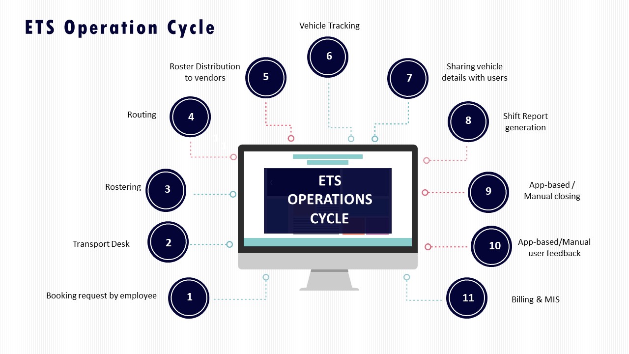
What should a leakage-control checklist include for supervisors—no-shows, ad-hoc approvals, manifest hygiene—so we’re not dependent on a few people maintaining spreadsheets?
B0366 Supervisor leakage control checklist — In India’s corporate EMS operations, what should a ‘leakage control checklist’ contain for day-to-day supervisors (no-shows, ad-hoc approvals, manifest hygiene, route adherence) so the program doesn’t depend on a few heroes maintaining spreadsheets?
A practical leakage control checklist for EMS supervisors in India must convert everyday risks like no‑shows, adhoc trips, bad manifests, and route deviations into simple, auditable checks per shift. The goal is to catch revenue and control leakages early at the command‑center level, so reliability does not depend on individual “heroes” or manual spreadsheets.
Supervisors need clear daily SOPs aligned to ETS operation cycles, routing tools, and centralized dashboards. Each checklist item should be verifiable in the EMS platform or command centre, not just “noted” in a logbook. Most organizations stabilize leakage when no‑show handling, adhoc approvals, manifest hygiene, and route adherence have explicit checks before, during, and after each shift.
A robust shift‑level leakage control checklist for supervisors should at minimum include:
- Rosters & Bookings. Verify that the ETS roster matches HRMS shift data for the day. Confirm booking cut‑off policy has been enforced. Flag manual additions outside cut‑off as exceptions with approver name/time.
- Vehicle–Route Assignment. Check that every scheduled trip has a tagged vendor vehicle and driver in the system. Ensure vehicle capacity is appropriate to planned Trip Fill Ratio targets to reduce dead mileage.
- Driver & Fleet Compliance Snapshot. Confirm all scheduled vehicles appear as “compliant” in the centralized compliance dashboard (valid permits, insurance, fitness, driver KYC/PSV current). Any override must be logged with supervisor ID and reason.
- Pre‑Shift Manifest Hygiene. Validate passenger manifests against HR master list. Remove resigned/transfer employees. Ensure only authorized employees, with correct gender tags and night‑shift rules, appear on manifests.
- Escort & Women‑Safety Rules. For night routes, confirm escorts and “female‑first / last‑drop” rules are correctly reflected in route plans. Flag any exception and record written approval from Security or HR.
- No‑Show & Cancellation Rules (Pre‑Dispatch). Before dispatch, review last‑minute cancellations and no‑shows from the employee app. Confirm withdrawal or pooling changes are updated in the system so billing does not include these seats.
- Ad‑Hoc Trip Approvals. Ensure every adhoc trip has a recorded requester, cost centre, and approver in the system. No trip should start on a phone call alone. Use the admin/transportation app’s request and approval workflow as a hard gate.
- GPS & App Health Check. At shift start, confirm all active vehicles are visible on the command‑centre map. If any GPS or app is offline, record the issue and ensure a backup tracking mode or manual duty slip is created before vehicle moves.
- Route Adherence Monitoring. During trips, monitor geo‑fence and route deviation alerts. Investigate any detours beyond approved corridors and capture driver explanation. Escalate repeated offenders via driver management and training SOPs.
- Live No‑Show Handling (On‑Route). When a no‑show occurs at pickup, ensure the driver records it in the driver app or via SOS/control panel. Supervisor should verify time‑stamped proof (call log/app status) before marking billable or non‑billable.
- Unplanned Detours / Extra Drops. Check for unscheduled stops or extra drop points against manifest. Any request from employees for “on the way” diversions should require supervisor approval and be tagged for billing or disciplinary action.
- Trip Closure Discipline. At end of each route, confirm trip closure in the system with actual times and odometer readings. Trips without proper closure cannot move to billing. Use e‑trip sheet features where available.
- Exception Log for Each Shift. Maintain a simple exception register inside the platform (or control‑room tool) covering: adhoc trips, manifest overrides, escort exceptions, GPS failures, and serious delays. Each entry must have root cause and owner.
- Billing Readiness Check. Before handing data to billing, quickly reconcile count of completed trips, cancelled trips, and no‑show‑only trips against the platform’s shift report. Any manual edit must be justified in remarks.
- Vendor Reconciliation Spot‑Check. For at least one route per vendor per shift, cross‑verify vendor duty slip vs system trip log (time, distance, passengers). Escalate discrepancies through vendor & statutory compliance channels.
- Safety & Incident Cross‑Check. Confirm all SOS triggers, alerts, or safety complaints during the shift have corresponding tickets with closure notes. Unclosed safety tickets must be blocked from billing until resolved.
- Driver Fatigue & Duty Cycle Check. For frequent drivers, verify they are within acceptable duty cycle norms according to safety and HSSE tools. Flag over‑duty patterns for roster correction to avoid incidents and hidden cost of breakdowns.
- Daily KPI Snapshots. Record shift‑level OTP%, Trip Adherence Rate, seat‑fill, and no‑show rate from the mobility dashboard. Store these snapshots centrally instead of local spreadsheets to gradually build a leakage and performance trend.
- Feedback & Complaint Loop. Ensure all negative feedback logged via employee app, call centre, or email is ticketed and linked to specific trips. Use this to identify repeat leakage patterns like fake no‑shows or habitual late arrivals.
This checklist is most effective when embedded into the command centre workflow and EMS tools described in the ETS Operation Cycle and Alert Supervision System. Supervisors should be required to digitally “check off” these items at pre‑shift, mid‑shift, and post‑shift stages, so leakage control becomes a routine process instead of hero‑driven spreadsheet work.
images:
How can we build a simple best/base/worst sensitivity view for the CFO—hybrid attendance, weather, Tier-2 constraints—without turning it into a big modeling exercise?
B0367 Board-ready sensitivity analysis — For India’s corporate ground transportation, how do you design sensitivity analysis that a CFO can actually use in board reviews—showing best/base/worst cases for hybrid attendance, weather disruptions, and Tier-2 constraints—without it becoming a complex modeling project?
To design sensitivity analysis that a CFO can use in a board review, the transport team should limit scope to 3–4 high‑impact variables, anchor them in existing trip/billing data, and present outcomes as simple, comparable scenarios rather than a complex model. The sensitivity analysis should express impacts in a small set of unit metrics that boards already understand, such as cost per employee trip, on‑time performance percentage, and EV utilization ratio, instead of exposing the underlying modeling logic.
The starting point is to fix a clean “base case” using one recent, representative month of employee mobility and corporate car rental data. The base case should lock in actual hybrid attendance patterns, current OTP%, cost per km, seat‑fill, and Tier‑2 versus metro trip mix. From there, the analysis can vary only a few drivers such as attendance volatility, weather‑related disruption days, and Tier‑2 share of trips, with each dimension tested at a low/medium/high level rather than on a continuous scale.
The CFO‑friendly design uses three aggregated scenarios rather than detailed matrices. A best case can assume higher seat‑fill, fewer disruption days, and stable Tier‑2 share. A base case can simply mirror the recent month. A worst case can assume elevated hybrid volatility, a short burst of heavy weather, and increased Tier‑2 exposure with lower fleet density. Each scenario should output the same small dashboard: cost per employee trip, total monthly cost band, OTP%, exception‑closure time, and any knock‑on EV or ESG impact such as emission intensity per trip.
This approach works when operational complexity is hidden behind simple levers. The transport and analytics teams can handle details like route optimization, dead mileage caps, and Tier‑2 vendor mix inside their own tools while only exposing the result bands to Finance. A common failure mode is trying to show every routing and vendor assumption to the board, which overwhelms non‑operational stakeholders and weakens the narrative. The more effective pattern is to pre‑agree the input ranges with Finance and Procurement, then lock the scenario templates so they can be reused in each board cycle.
A minimal, reusable structure usually includes:
- A one‑page base case summary with current KPIs and exposure breakdown for metros versus Tier‑2 cities.
- A three‑column scenario table where each column shows best/base/worst values for unit costs, OTP, and disruption‑day counts.
- A short note on operational levers that would be pulled in the worst case, such as buffer fleet activation, EV versus diesel mix shifts, or temporary routing changes.
This keeps the sensitivity analysis aligned with outcome‑linked procurement metrics and allows the CFO to discuss risk bands and trade‑offs without needing to interpret a complex model.
How can we link dead-mile reduction to employee experience and attendance so HR doesn’t feel Finance is cutting cost at the expense of employees?
B0368 Dead-mile savings with HR trust — In India’s corporate EMS programs, what is the most defensible way to link reductions in dead miles to employee experience and attendance outcomes, so HR doesn’t feel Finance is optimizing purely for cost at the expense of people?
In Indian corporate EMS programs, the most defensible way to link dead-mile reduction with employee experience and attendance is to treat “less dead mileage” as an enabler of higher on-time performance and safety, then prove this link with shared KPIs that HR and Finance co-own. Dead-mile cuts are framed as freeing capacity for better routing, more buffers, and safer, more predictable commutes, not just as a fuel-saving exercise.
Dead mileage directly affects route design, buffer times, and driver duty cycles. Lower dead miles allow the same fleet to cover live trips with more predictable shift windowing and less driver fatigue, which typically improves on-time performance and trip adherence. Higher on-time performance and stable routing patterns support better attendance and reduce night-shift anxiety, particularly for women employees subject to escort and routing rules. HR can position this as reliability and safety by design, not cost cutting.
Finance, HR, and the transport head can jointly define a compact KPI set that always reports dead mileage alongside service and people outcomes. For example, HR tracks a Commute Experience Index, complaint volumes, and late-login incidents, while operations tracks OTP%, Trip Adherence Rate, and Driver Fatigue Index, and Finance tracks Cost per Employee Trip. Any dead-mile reduction initiative moves forward only when OTP and CEI are stable or improving, and when night-shift and women-safety policies remain fully compliant.
A practical safeguard is to run A/B or pilot routes where dynamic routing and seat-fill optimization reduce dead miles, while a command center monitors exceptions, SOS triggers, and incident logs in real time. If OTP, complaint closure SLAs, and safety incident rates improve or hold steady along with reduced dead mileage, HR gains defensible evidence that cost optimization is aligned with duty of care and attendance stability, not working against it.
How do we make sure EMS invoices reflect actual seat-fill and approved exceptions—not just vendor summaries—so month-end isn’t a recurring negotiation?
B0369 Invoice tied to seat-fill — For India’s EMS billing and SLA governance, how can Finance ensure the invoice reflects real seat-fill performance and approved exceptions (instead of vendor-reported aggregates), so month-end closure doesn’t become a negotiation every cycle?
Finance teams can anchor EMS billing and SLA governance on system-of-record trip data that is tied to seat-level manifests, policy rules, and exception approvals, rather than on vendor-reported summaries. This shifts month-end from a negotiated aggregate to a reconciled output based on a shared trip ledger, seat-fill calculations, and pre-defined exception workflows.
To do this effectively, organizations need EMS platforms that capture seat-level bookings, boarding, and no-shows, and that compute Trip Fill Ratio and Cost per Employee Trip directly from manifests. Vendor invoices are then generated or validated using this same data set, which reduces the scope for manual interpretation and disputes. Outcome-linked procurement becomes feasible only when seat-fill, OTP, and exception closure times are derived from a common, auditable data layer.
A common failure mode is fragmented data, where HRMS rosters, transport desk sheets, and vendor logs do not match. In such environments, Finance is forced into month-end negotiations because there is no agreed source of truth for who actually travelled, on which route, and under what approved exception. Another typical gap is the absence of codified exception rules, which leaves waivers and additions to ad-hoc email approvals that are hard to reconcile against trip-level billing lines.
Finance can reduce friction by insisting on a few operational safeguards that are agreed upfront with HR, Transport, and Procurement:
- A consolidated EMS trip ledger with seat-level manifests and timestamps as the billing baseline.
- Configured commercial rules in the platform that link payable units to seat-fill, OTP, and defined SLA outcomes.
- Formal exception workflows in the system, with approver identity, reason codes, and validity windows, so exceptions are machine-readable.
- Standard invoice formats that reference trip IDs and exception IDs, allowing automated reconciliation to Finance and HRMS data.
When these elements are in place, EMS billing reflects real utilization and governed exceptions, and month-end closure becomes a verification exercise rather than a repeated commercial debate.
Even if OTP looks fine, what issues still cause attendance volatility, and how can we spot them early using route and manifest data?
B0370 Attendance volatility despite OTP — In India’s shift-based employee transport, what operational behaviors typically cause ‘attendance volatility’ even when OTP metrics look acceptable, and how do you detect those patterns early using route and manifest data?
In India’s shift-based employee transport, attendance volatility often comes from micro-failures in routing, boarding, and perceived safety that do not show up in high-level OTP%.
Early detection depends on analyzing route- and manifest-level patterns such as who is repeatedly late-boarded, frequently rerouted, or exposed to higher-risk trip conditions.
Many organizations see “on-time” vehicles at the gate while employees still struggle to board in time.
A common failure mode is last-minute dynamic routing that keeps overall OTP within SLA but increases dead mileage and compresses pick-up windows, which reduces effective boarding time for specific clusters.
Another pattern is repeated re-assignment of certain employees to low-fill or edge routes, which increases travel time and fatigue and quietly drives drop in Commute Experience Index and then attendance.
Women on late-night shifts may experience more route deviations or escort non-compliance, which creates perceived risk and leads to discretionary absenteeism even if official incident numbers are low.
Transport teams can detect these hidden behaviours by treating the route and manifest as primary signals rather than relying only on trip-level OTP aggregates.
The key is to correlate individual employee manifests, route adherence audits, and trip lifecycle data with outcomes such as no‑show rate, late login flags, and complaint tags.
Useful early-warning checks include:
- Employee-level sequence drift. Track how often an employee’s pick-up sequence on a given route changes from its baseline pattern. Rising “sequence volatility” for a cohort is an indicator of unstable routing that can lead to churn and absenteeism.
- Compressed pick-up windows. Measure the gap between “planned” vs “actual” arrival at each stop and the scheduled shift start. If the median buffer for a team falls below a defined threshold, attendance volatility typically rises even when trip OTP at facility gate remains within SLA.
- Repeated partial route adherence. Use route adherence audits to flag specific routes where actual GPS traces systematically diverge from the approved path, especially on late-night and women-first routes. Employees on these manifests are more likely to self-select out of certain shifts.
- No-show clustering by route and timeband. Monitor no-show rate per route, timeband, and seat position on the manifest. If a subset of routes shows elevated no-shows despite acceptable OTP, it usually reflects perceived unreliability or discomfort on those paths.
- High re-routing and trip-cancellation frequency. Count how many times a route is re-planned or a pick-up is re-assigned in the last hour before shift. Frequent last-minute changes erode trust and create a pattern of “soft exits” from marginal shifts.
Most stable operations build these checks into the command center’s dashboard.
They use a centralized NOC to watch Vehicle Utilization Index, Trip Fill Ratio, dead mileage, and OTP alongside per-employee manifest stability, route adherence score, and no-show trend lines.
When any one route, driver, or cluster shows rising sequence volatility, compressed buffers, or no-show spikes, transport heads can intervene early with targeted routing fixes, driver coaching, or capacity rebalancing before HR sees a broader attendance problem.
How do we stop vendors from showing lower CET/CPK but pushing costs into add-ons like waiting or night allowances, and what contract controls keep total cost predictable?
B0371 Prevent add-on cost gaming — For India’s corporate EMS procurement, how do you prevent vendors from gaming CET/CPK by shifting costs into add-ons (waiting, tolls, parking, night allowances), and what contract controls keep total cost predictable without constant disputes?
In India’s corporate EMS, organizations prevent vendors from gaming cost per employee trip (CET) and cost per kilometer (CPK) by moving to all‑in, clearly defined commercial buckets, hard caps on pass‑throughs, and strict linkage of invoices to auditable trip data. The most effective contracts treat tolls, parking, waiting, and night allowances as governed line items with rules and ceilings, not open‑ended add‑ons.
A common failure mode is defining only a low base CPK or per‑trip rate and leaving “extras” loosely worded. Vendors then recover margins through uncontrolled waiting, adhoc toll claims, and night charges. This usually results in CET volatility, frequent Finance–vendor disputes, and manual reconciliation overhead for Procurement and Transport.
Contract structures that maintain predictable total cost typically include itemized but constrained components. Organizations define inclusive scope for the base rate, then specify when waiting, tolls, and parking are payable, how they are calculated, and what caps apply per trip, per shift, or per month. Night allowances and escort costs are linked to shift windows and pre‑approved rosters instead of being claimed ad hoc.
To keep arguments down, most mature buyers insist on technology‑linked evidence. Invoice lines must reconcile with GPS trip logs, geo‑tagged duty slips, and system‑recorded wait times from the EMS platform or command center, rather than vendor spreadsheets. Centralized billing and standardized models (for example, fixed packages versus per‑km versus trip‑based) further reduce room for interpretation.
Practical contract controls that improve predictability and reduce gaming include:
- Clear definition of “what is included” in base CET/CPK versus what is truly exceptional.
- Pre‑approved and capped schedules for waiting, tolls, parking, and night/escort allowances.
- Mandatory alignment of every billed extra to trip IDs and telematics data.
- Standard commercial models and tariff mapping across all locations and vendors, governed by a single SLA and escalation matrix.
How can we measure month-end reconciliation toil—hours spent, exceptions per 1,000 trips—and use it to build a Finance-ready case for automating leakage controls?
B0372 Quantify reconciliation toil savings — In India’s corporate employee transport operations, what’s a realistic way to measure ‘toil’ in month-end reconciliation (hours spent, exceptions per 1,000 trips) and link that reduction to a Finance-ready value case for automating leakage controls?
In corporate employee transport operations, “toil” in month-end reconciliation can be measured as a combination of human hours spent on closure activities and exception volume per 1,000 trips, and this quantified baseline can then be converted into a Finance-ready value case by assigning cost to those hours, to the leakage they are masking, and to audit risk they create.
A pragmatic approach is to treat reconciliation as a recurring operational process with a small, fixed metric set. Organizations can log the number of people involved in billing closure, the hours each spends on transport-related reconciliation, and the number of exceptions they touch. Exceptions typically cover items like trip mismatches between vendor and system, dead mileage disputes, tariff mapping errors, manual rate overrides, and credit/debit notes raised after invoice submission. For a given month, total reconciliation hours and total exceptions can be divided by total completed trips to produce “hours per 1,000 trips” and “exceptions per 1,000 trips” as stable operational KPIs.
Linking this to a Finance-ready automation case is easier if each metric is tied to unit economics and risk. Reconciliation hours can be multiplied by fully loaded FTE cost and by the cycle time impact on cash application to show opex burden. Exceptions can be categorized into value-bearing (e.g., rate disputes, dead mileage) and non-value-bearing (pure data quality issues) and then analyzed for average rupee impact per exception. That lets Finance see how many rupees per 1,000 trips are in play due to leakage, reversals, and disputes.
Once automation of leakage controls is introduced, the same KPIs can be tracked for at least two or three reconciliation cycles. Typical automated controls include tariff mapping engines tied to service catalogs, trip ledger consolidation from the routing platform, automated tax calculations aligned with centralized billing, and rule-based tolerance thresholds for dead mileage or waiting time. If hours per 1,000 trips fall, and exceptions per 1,000 trips decline while SLA breach rate and cost-per-trip remain stable or improve, Finance can attribute quantified savings to lower manual effort, reduced leakage, and lower audit exposure, and treat these as recurring gains rather than one-time optimization.
A minimal but robust monthly lens that Finance teams can work with is:
- Total transport trips vs total “billing-touch” hours to derive hours per 1,000 trips.
- Total exceptions logged vs total trips to derive exceptions per 1,000 trips, segmented by type and value impact.
- Difference between system-calculated charges and final invoiced amount (positive and negative) as rupee leakage per 1,000 trips.
- Cycle time from trip month-end to invoice approval as a proxy for working-capital and audit pressure.
During heavy weather disruptions, how do Ops and Finance decide if we should relax seat-fill targets, and how do we document it so it won’t get flagged later?
B0373 Govern seat-fill exceptions in disruptions — For India’s corporate EMS programs, when weather disruptions cause repeated route failures, how do Operations and Finance decide whether to temporarily relax seat-fill targets, and how do they document that decision so auditors don’t flag ‘policy exceptions’ later?
For Indian corporate EMS programs, Operations and Finance typically relax seat‑fill targets only when they can clearly show that maintaining standard pooling would jeopardize reliability or safety, and they document this as a governed, time‑bound exception linked to a specific disruption event. The decision is framed as a controlled business continuity measure, not an ad‑hoc commercial change, and is backed by data, approvals, and explicit audit trails.
Operations first establishes that weather is directly driving route failures. Operations teams use command‑center data such as On‑Time Performance (OTP%), Trip Adherence Rate, exception closure times, and no‑show or partial‑completion patterns during the disruption window. They correlate these with external triggers like monsoon alerts or flooding, and with routing constraints such as closed roads and traffic bottlenecks. This evidence shows that strict seat‑fill and dead‑mileage targets now conflict with shift adherence and duty‑of‑care obligations.
Finance evaluates the cost and control impact of relaxing seat‑fill. Finance models the delta in Cost per Employee Trip and Cost per Kilometer under lower pooling, and compares it to cost of failed shifts, overtime, or productivity loss. Finance checks that the EMS commercial model and vendor contracts (including penalties and incentives) can accommodate a temporary deviation without breaking the overall TCO narrative.
To avoid future audit flags, the joint decision is captured inside existing governance and continuity structures, not outside them. Typical documentation elements include:
- A dated Business Continuity or emergency operations note that defines the disruption, affected locations, and expected duration.
- A formal, signed decision record from the mobility governance forum or an equivalent committee that states which KPIs are being relaxed (for example, Trip Fill Ratio or dead‑mile caps), for how long, and under what thresholds OTP and safety take clear precedence.
- Updates to the mobility risk register and EMS operating playbook that classify this as a “temporary emergency routing protocol,” mapping it to existing business continuity and safety obligations.
- Tagged data in the mobility platform or billing system so all impacted trips are marked with an “exception code” tied to the weather event, allowing trip‑level analytics, billing reconciliation, and future audits to separate these trips from normal operations.
- A short post‑event review that records OTP%, incidents, safety performance, and cost impact versus baseline, and confirms the reversion point when standard seat‑fill and routing policies were restored.
In practice, Operations owns the real‑time decision and execution under a documented business continuity playbook, while Finance and Procurement own the commercial and policy framing. Security or HSSE functions reinforce that lower pooling is being used to uphold statutory safety, night‑shift, and duty‑of‑care obligations during the disruption. This integrated approach ensures auditors see a controlled, traceable use of emergency levers rather than unmanaged “policy exceptions.”